Discounting at the beginning and at the end of the period. What is and why the discount rate in ordinary life - a simple calculation, scope, practical application
Notes:
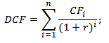
1. The discount factor (discount factor) is set by the formula:
Where r is the discount rate, %; t is the settlement period, years.
2. ![]()
![]()
![]()
In a similar manner, the discount factor for project No. 2 is determined.
Based on the data in Table. 10.6, determine the net present effect (NPE) for investment projects:
NPI1 \u003d 17368 - 14000 - 3368 thousand rubles;
NPI2 \u003d 16442 - 13400 \u003d 3042 thousand rubles.
So, a comparison of NPI indicators for projects confirms that the first of them is more effective than the second. NPI on it for 326 thousand rubles. (3368 -- 3042), or 9.7% more than in the second project. However, under project No. 1, the amount of capital investments for 600 thousand rubles. (14,000 - 13,400), or 4.3%, higher than in the second project, and their return in the form of future cash flow is lower than in project No. 2 by 2,000 thousand rubles. (20,000 - 22,000). In the case of the implementation of project No. 1, the investor needs to find additional funding (internal or external) in the amount of 600 thousand rubles. Therefore, he must choose for himself the most appropriate option, taking into account the available financial possibilities.
It should be noted that the NPI indicator is absolute, so it can be summed up and compared with other similar projects. In addition, it can be used not only for a comparative assessment of the effectiveness of projects at the preliminary stage of their consideration, but also as a criterion for the expediency of their implementation. Projects for which the NPI is negative or equal to zero are unacceptable for the investor, since they will not bring him additional income on invested capital. Projects with a positive NPI increase the investor's initial capital advance.
The CPE method is not an absolutely correct criterion for:
Fluctuations in the discount rate during the project implementation period due to changes in economic conditions in the investment goods market;
Choosing between a project with a large initial capital cost and a project with a significantly lower investment (3 million and 500 thousand rubles); it is obvious that if the influx Money will not be, then under the first project the enterprise will lose 6 times more than under the second one;
Choosing between a project with a large NPI and a long payback period and a project with a lower NPI and short term cost recovery (up to one year). Consequently, the NPE method does not allow to judge the profitability threshold and the margin of financial strength;
The choice of discount rate, especially in the conditions of an unstable Russian economy (rates bank interest, weighted average cost of capital, etc.).
Despite the noted shortcomings, this method (NPV) is recognized in international practice as the most reliable in the system of performance evaluation criteria. investment projects.
The indicator - discounted yield index (FIR) is calculated by the formula:
![]() (144)
(144)
where HC is the present value of cash flows; I - the amount of investments aimed at the implementation of the project (if the investments are at different times, it is also reduced to the present value).
Using the data for two projects, we determine the discounted profitability index for them:
DID1=1.241 (17,368/14,000);
DID2=1.241 (17,368/14,000);
Therefore, according to this parameter, the efficiency of the projects is approximately the same. If the value of the yield index is less than or equal to one, then the project is rejected, since it will not bring the investor additional income. Projects with a value of this indicator greater than one are accepted for implementation. It should be noted that with the growth of the absolute value of NPE (in the numerator of formula 144), the value of the discounted profitability index also increases, and vice versa. At zero NPI, the yield index is always equal to one. This means that only one of them can be taken as a criterion for the implementation of the project - NPI or profitability index. In practice, when comparative evaluation recommend considering both indicators and making the right investment decision.
In the article we will talk in detail about discounting cash flows, the calculation and analysis formula in Excel.
Discounting cash flows. Definition
Cash flow discounting (English Discounted cash flow, DCF, discounted value) is the reduction of the value of future (expected) cash payments to the current moment in time. Discounting cash flows is based on the important economic law of diminishing value of money. In other words, over time, money loses its value compared to the current one, so it is necessary to take the current moment of assessment and all future ones as a starting point. cash receipts(profit/loss) result to date. For this purpose, a discount factor is used.
How to calculate the discount factor?
Discount coefficient is used to convert future earnings to present value by multiplying the discount factor and the cash flows. The formula for calculating the discount factor is shown below:
where: r is the discount rate, i is the number of the time period.
 |
★ |
Discounting cash flows. Calculation formula
DCF( discounted cash flow– discounted cash flow;
CF ( Cashflow) - cash flow in time period I;
r is the discount rate (rate of return);
n is the number of time periods for which cash flows appear.
The key element in the discounted cash flow formula is the discount rate. The discount rate shows what rate of return an investor should expect when investing in a particular investment project. The discount rate uses many factors that depend on the object of assessment, and may include: inflation component, return on risk-free assets, additional rate of return for risk, refinancing rate, weighted average cost of capital, interest on bank deposits etc.
Calculating the rate of return (r) for discounting cash flows
There are enough various ways and methods for estimating the discount rate (rate of return) in investment analysis. Let us consider in more detail the advantages and disadvantages of some methods for calculating the rate of return. This analysis is presented in the table below.
|
Methods for estimating the discount rate |
Advantages |
Flaws |
| CAPM Models | Ability to account for market risk | One-factor, the need for the presence of ordinary shares in the stock market |
| Gordon Model | Ease of calculation | The need for ordinary shares and constant dividend payments |
| Weighted average cost of capital (WACC) model | Accounting for the rate of return of both equity and debt capital | Difficulty in assessing returns equity |
| Model ROA, ROE, ROCE, ROACE | Ability to take into account the return on capital of the project | Not taking into account additional macro, micro risk factors |
| E/P method | Accounting for the market risk of the project | Availability of quotes on the stock market |
| Method for estimating risk premiums | Using Additional Risk Criteria in Estimating the Discount Rate | Subjectivity of risk premium estimation |
| Judgment-Based Appraisal Method | Possibility to take into account weakly formalized project risk factors | Subjectivity of expert assessment |
You can learn more about the approaches to calculating the discount rate in the article "".
|
★ (calculation of Sharpe, Sortino, Trainor, Kalmar, Modiglanchi beta, VaR ratios) + rate movement forecasting |
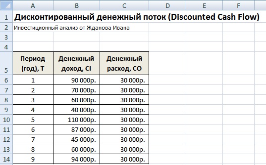
Example of calculating discounted cash flow in Excel
In order to calculate discounted cash flows, it is necessary for the selected time period (in our case, annual intervals) to describe in detail all the expected positive and negative cash payments (CI - Cashinflow, CO CashOutflow). The following payments are taken for cash flows in valuation practice:
- Net operating income;
- Net cash flow excluding operating costs, land tax and facility refurbishment;
- Taxable income.
In domestic practice, as a rule, a period of 3-5 years is used; in foreign practice, the assessment period is 5-10 years. The entered data is the basis for further calculation. The figure below shows an example of entering initial data in Excel.
The next step is to calculate the cash flow for each of the time periods (column D). One of the key tasks in assessing cash flows is to calculate the discount rate, in our case it is 25%. And was obtained by the following formula:
Discount rate= Risk free rate + Risk premium
The key rate of the Central Bank of the Russian Federation was taken as the risk-free rate. The key rate of the Central Bank of the Russian Federation is currently 15% and the premium for risks (production, technological, innovative, etc.) was calculated by an expert at the level of 10%. The key rate reflects the return on a risk-free asset, and the risk premium shows an additional rate of return on the existing risks of the project.
You can learn more about calculating the risk-free rate in the following article: ""
After that, it is necessary to bring the received cash flows to the initial period, that is, multiply them by the discount factor. As a result, the sum of all discounted cash flows will give the discounted value investment object. The calculation formulas will be as follows:
Cash flow (CF)=B6-C6
Discounted cash flow (DCF)= D6/(1+$C$3)^A6
Total discounted cash flow (DCF)= SUM(E6:E14)

As a result of the calculation, we received the discounted value of all cash flows (DCF) equal to 150,981 rubles. This cash flow has a positive value, which indicates the possibility of further analysis. When conducting investment analysis it is necessary to compare the final values of the discounted cash flow for various alternative projects, this will allow them to be ranked according to the degree of attractiveness and efficiency in creating value.
Investment analysis methods using discounted cash flows
It should be noted that discounted cash flow (DCF) in its calculation formula is very similar to net present value (NPV). The main difference lies in the inclusion of the original investment costs into the NPV formula.
Discounted cash flow (DCF) is used in many methods for evaluating the effectiveness of investment projects. Due to the fact that these methods use discounted cash flows, they are called dynamic.
- Dynamic methods for evaluating investment projects
- Net present value (NPV,Netpresentvalue)
- internal norm arrived ( IRR, Internal Rate of Return)
- profitability index (PI, Profitability index)
- Annuity equivalent (NUS, Net Uniform Series)
- net rate of return ( NRR, Net Rate of Return)
- Net future value ( nfv,NetFuturevalue)
- Discounted payback period (DPP,Discountedpayback period)
You can learn more about the methods for calculating the effectiveness of investment projects in the article "".
Besides only discounting cash flows, there are more sophisticated methods that additionally take into account the reinvestment of cash payments.
- Modified net norm profitability ( MNPV, Modified Net Rate of Return)
- Modified rate of return ( MIRR, Modified Internal Rate of Return)
- Modified net present value ( MNPV,modifiedpresentvalue)
|
★ (calculation of Sharpe, Sortino, Trainor, Kalmar, Modiglanchi beta, VaR ratios) + rate movement forecasting |
Advantages and Disadvantages of the DCF Measure of Discounted Cash Flows
+) The use of the discount rate is an undoubted advantage of this method, as it allows you to bring future payments to the current value and take into account possible factors risk assessment investment attractiveness project.
-) The disadvantages include the difficulty of predicting future cash flows for an investment project. In addition, it is difficult to reflect changes in the external environment in the discount rate.
Summary
Cash flow discounting is the basis for calculating many coefficients for evaluating the investment attractiveness of a project. We analyzed the example of the algorithm for calculating discounted cash flows in Excel, their existing advantages and disadvantages. Ivan Zhdanov was with you, thank you for your attention.
Highly specialized material for professional investors
and students of the Fin-plan course "".
Financial and economic calculations are most often associated with the assessment of time-distributed cash flows. Actually for these purposes, and need a discount rate. From the point of view of financial mathematics and investment theory, this indicator is one of the key. Methods are built on it. investment appraisal business based on the concept of cash flows, with its help, a dynamic assessment of the effectiveness of investments, both real and stock, is carried out. To date, there are already more than a dozen ways to select or calculate this value. Mastering these methods allows professional investor make smarter and more timely decisions.
But, before moving on to the methods of justifying this rate, let's look at its economic and mathematical essence. Actually, two approaches are applied to the definition of the term "discount rate": conditionally mathematical (or process), as well as economic.
The classic definition of the discount rate stems from the well-known monetary axiom: “Money today is worth more than money tomorrow.” Hence, the discount rate is a certain percentage that allows you to bring the cost of future cash flows to their current cost equivalent. The fact is that many factors influence the depreciation of future income: inflation; risks of not receiving or not receiving income; lost profit arising from the appearance of a more profitable alternative investment opportunity in the process of implementing a decision already made by the investor; systemic factors and others.
By applying a discount rate in their calculations, an investor discounts, or discounts, expected future cash income to the current point in time, thereby taking into account the above factors. Discounting also allows the investor to analyze cash flows over time.
In this case, the discount rate and the discount factor should not be confused. The discount factor is usually used in the calculation process as a kind of intermediate value calculated on the basis of the discount rate according to the formula:
where t is the number of the forecast period in which cash flows are expected.
The product of the future value of the cash flow and the discount factor shows the current equivalent of the expected income. However, the mathematical approach does not explain how the discount rate itself is calculated.
For these purposes, it is used economic principle, according to which the discount rate is some alternative return comparable investments with the same level risk. A rational investor, making a decision to invest money, will agree to the implementation of his "project" only if its profitability turns out to be higher than the alternative and available on the market. This is not an easy task, since it is very difficult to compare investment options by level of risk, especially in the absence of information. In the theory of investment decision making, this problem is solved by decomposing the discount rate into two components - the risk-free rate and risks:
The risk-free rate of return is the same for all investors and is subject only to the risks of the economic system. The remaining risks are assessed by the investor independently, as a rule, on the basis of an expert assessment.
There are many models to justify the discount rate, but all of them in one way or another correspond to this basic fundamental principle.
Thus, the discount rate is always the sum of the risk-free rate and the total investment risk specific investment asset. The starting point for this calculation is the risk-free rate.
risk free rate
The risk-free rate (or risk-free rate of return) is the expected rate of return on assets that have zero intrinsic financial risk. In other words, this is the return on absolutely reliable options for investing money, for example, on financial instruments, the profitability of which is guaranteed by the state. We emphasize that even for absolutely reliable financial investments absolute risk cannot be absent (in this case, the rate of return would also tend to zero). The risk-free rate contains the risk factors of the economic system itself, risks that no investor can influence: macroeconomic factors, political events, changes in legislation, extraordinary anthropogenic and natural events, etc.
Therefore, the risk-free rate reflects the lowest possible return acceptable to the investor. The investor must choose the risk-free rate for himself. Can count average value rates from several options for potentially risk-free investments.
When choosing a risk-free rate, an investor should take into account the comparability of his investments with a risk-free option according to such criteria as:
Scale or total cost of investment.
Investment period or investment horizon.
The physical possibility of investing in a risk-free asset.
Equivalence of denomination of rates in currency, and others.
Rates of return on fixed-term ruble deposits in banks of the highest reliability category. In Russia, such banks include Sberbank, VTB, Gazprombank, Alfa-Bank, Russian Agricultural Bank and a number of others, a list of which can be viewed on the website Central Bank RF. When choosing a risk-free rate in this way, it is necessary to take into account the comparability of the investment period and the period of fixing the rate on deposits.
Let's take an example. We use the data of the website of the Central Bank of the Russian Federation. As of August 2017, the weighted average interest rates on deposits in rubles for up to 1 year amounted to 6.77%. This rate is risk-free for most investors who invest for up to 1 year;
Yield on Russian government debt financial instruments. In this case, the risk-free rate is fixed in the form of yield on (OFZ). These debt securities are issued and guaranteed by the Ministry of Finance of the Russian Federation, therefore they are considered the most reliable financial asset in RF. With a maturity of 1 year, OFZ rates currently range from 7.5% to 8.5%.
Level of return on foreign government securities. In this case, the risk-free rate is equal to the yield on US government bonds with maturities ranging from 1 to 30 years. Traditionally, the US economy is international rating agencies estimated at highest level reliability, and, consequently, the yield of their government bonds and is recognized as risk-free. However, it should be taken into account that the risk-free rate in this case is denominated in dollars and not in rubles. Therefore, for the analysis of investments in rubles, an additional adjustment for the so-called country risk is necessary;
Yield on Russian government Eurobonds. This risk-free rate is also denominated in dollar terms.
The key rate of the Central Bank of the Russian Federation. At the time of this writing, the key rate is 9.0%. It is believed that this rate reflects the price of money in the economy. An increase in this rate entails an increase in the cost of a loan and is a consequence of an increase in risks. This tool should be used with great care, as it is still a directive, not a market indicator.
Interbank lending market rates. These rates are indicative and more acceptable than key rate. Monitoring and a list of these rates are again presented on the website of the Central Bank of the Russian Federation. For example, as of August 2017: MIACR 8.34%; RUONIA 8.22%, MosPrime Rate 8.99% (1 day); ROISfix 8.98% (1 week). All these rates are short-term and represent the yield on lending operations of the most reliable banks.
Discount rate calculation
To calculate the discount rate, the risk-free rate should be increased by the risk premium that the investor assumes when making certain investments. It is impossible to assess all risks, so the investor must independently decide which risks and how should be taken into account.
The following parameters have the greatest influence on the value of the risk premium and, ultimately, the discount rate:
The size of the issuing company and the stage of its life cycle.
The nature of the liquidity of the company's shares in the market and their volatility. The most liquid stocks generate the least risk;
Financial condition share issuer. stable financial position increases the adequacy and accuracy of forecasting the company's cash flow;
Business reputation and perception of the company by the market, investors' expectations regarding the company;
Industry affiliation and risks inherent in this industry;
The degree of exposure of the activity of the issuing company to macroeconomic conditions: inflation, fluctuations in interest rates and exchange rates etc.
A separate group of risks includes the so-called country risks, that is, the risks of investing in the economy of a particular state, for example, Russia. As a rule, country risks are already included in the risk-free rate, if the rate itself and the risk-free yield are denominated in the same currencies. If the risk-free return is in dollar terms, and the discount rate is needed in rubles, then it will be necessary to add country risk as well.
This is just a short list of risk factors that can be taken into account in the discount rate. Actually, depending on the method of assessing investment risks, the methods for calculating the discount rate differ.
Let us briefly consider the main methods for justifying the discount rate. To date, more than a dozen methods for determining this indicator have been classified, but they are all grouped as follows (from simple to complex):
Conditionally "intuitive" - based rather on the psychological motives of the investor, his personal beliefs and expectations.
Expert, or qualitative - based on the opinion of one or a group of specialists.
Analytical - based on statistics and market data.
Mathematical, or quantitative - require mathematical modeling and the possession of relevant knowledge.
An "intuitive" way to determine the discount rate
Compared to other methods this way is the simplest. The choice of the discount rate in this case is not mathematically justified in any way and represents only the desire of the investor, or his preference for the level of profitability of his investments. An investor can rely on his previous experience, or on the profitability of similar investments (not necessarily his own), if he knows the information about the profitability of alternative investments.
Most often, the discount rate is "intuitively" calculated approximately by multiplying the risk-free rate (as a rule, this is just the deposit rate or OFZ) by some adjustment factor of 1.5, or 2, etc. Thus, the investor, as it were, “estimates” the level of risks for himself.
For example, when calculating the discounted cash flows and fair value of companies in which we plan to invest, we usually use the following rate: average rate on deposits, multiplied by 2 if we are talking about blue chips and apply higher coefficients if we are talking about companies of the 2nd and 3rd tier.
This method is the simplest practice for a private investor and is used even in large investment funds experienced analysts, but he is not held in high esteem among academic economists, because he allows for “subjectivity”. In this regard, in this article we will give an overview of other methods for determining the discount rate.
Calculation of the discount rate based on expert judgment
The expert method is used when investments involve investing in shares of companies in new industries or activities, start-ups or venture funds, and also when there are no adequate market statistics or financial information about the issuing company.
The expert method for determining the discount rate consists in polling and averaging the subjective opinions of various experts about the level, for example, the expected return on specific investments. The disadvantage of this approach is the relatively high proportion of subjectivity.
You can increase the accuracy of calculations and somewhat level out subjective assessments by decomposing the rate into a risk-free level and risks. The investor chooses the risk-free rate on his own, and the assessment of the level of investment risks, the approximate content of which we described earlier, is already carried out by experts.
The method is well applicable for investment teams that employ investment experts of various profiles (currency, industry, raw materials, etc.).
Calculation of the discount rate by analytical methods
There are many analytical ways to justify the discount rate. All of them are based on the theory of economics of the firm and financial analysis, financial mathematics and business valuation principles. Let's give some examples.
Calculation of the discount rate based on profitability indicators
In this case, the discount rate is justified on the basis of various profitability indicators, which, in turn, are calculated according to the data and . As a base indicator, return on equity (ROE, Return On Equity) is used, but there may be others, for example, return on assets (ROA, Return On Assets).
Most often used to evaluate new investment projects within an existing business, where the nearest alternative rate profitability is precisely the profitability of the current business.
Calculation of the discount rate based on the Gordon model (model of constant growth of dividends)
This method of calculating the discount rate is acceptable for companies that pay dividends on their shares. This method assumes the fulfillment of several conditions: the payment and positive dynamics of dividends, the absence of restrictions on the life of the business, and the stable growth of the company's income.
The discount rate in this case is equal to the expected return on equity of the company and is calculated by the formula:
This method is applicable to the evaluation of investments in new projects of the company, by the shareholders of this business, who do not control profits, but receive only dividends.
Calculation of the discount rate by quantitative analysis methods
From the point of view of investment theory, these methods and their variations are the main and most accurate. Despite the many varieties, all these methods can be reduced to three groups:
Models of cumulative construction.
Capital Asset Pricing Model (CAPM).
Models of the weighted average cost of capital WACC (Weighted Average Cost of Capital).
Most of these models are quite complex, requiring a certain mathematical or economic skill. We'll consider general principles and basic calculation models.
Cumulative building model
Within the framework of this method, the discount rate is the sum of the risk-free rate of expected return and the total investment risk for all types of risk. The method of substantiating the discount rate based on risk premiums to the risk-free level of return is used when it is difficult or impossible to evaluate the relationship between risk and return on investment in the analyzed business using mathematical statistics. V general view the calculation formula looks like this:
Capital asset pricing model CAPM
The author of this model is the Nobel laureate in economics W. Sharp. The logic of this model does not differ from the previous one (the rate of return is the sum of the risk-free rate and risks), the method of assessing investment risk is different.
This model is considered fundamental, since it establishes the dependence of profitability on the degree of its exposure external factors market risk. This relationship is assessed through the so-called "beta" coefficient, which is essentially a measure of the elasticity of an asset's return to a change in the average market return of similar assets in the market. In general, the CAPM model is described by the formula:
Where β is the “beta” coefficient, a measure of systematic risk, the degree of dependence of the assessed asset on the risks of the economic system itself, and the average market return is the average return on the market for similar investment assets.
If the "beta" coefficient is higher than 1, then the asset is "aggressive" (more profitable, changing faster than the market, but also more risky in relation to analogues in the market). If the "beta" coefficient is below 1, then the asset is "passive" or "protective" (less profitable, but also less risky). If the "beta" coefficient is equal to 1, then the asset is "indifferent" (its profitability changes in parallel with the market).
Calculation of the discount rate based on the WACC model
Estimating the discount rate based on the company's weighted average cost of capital allows you to estimate the cost of all sources of financing for its activities. This indicator reflects the actual cost of the company to pay for borrowed capital, share capital, other sources weighted by their share in the total liability structure. If the company's actual return is above WACC, then it generates some added value for its shareholders, and vice versa. That is why the WACC indicator is also considered as a barrier value of the required return for the company's investors, that is, the discount rate.
The calculation of the WACC indicator is carried out according to the formula:

Of course, the range of methods for justifying the discount rate is quite wide. We have described only the main methods most often used by investors in a given situation. As we said earlier in our practice, we use the simplest, but quite effective "intuitive" way to determine the rate. The choice of a specific method always remains with the investor. You can learn the whole process of making investment decisions in practice in our courses at. We teach deep analytics techniques already at the second level of training, at advanced training courses for practicing investors. You can evaluate the quality of our training and take the first steps in investing by signing up for ours.
If the article was useful to you, like and share it with your friends!
Profitable investment to you!
The factor FM2(r,k) = l/(l+r)k is called the discount factor for a single payment, its values are also tabulated. The economic meaning of the discount factor FM2(r,k) is as follows: it shows the current price of one monetary unit of the future, i.e., what is one monetary unit (for example, one ruble) circulating in the business sphere after k periods from the moment of calculation, at a given interest rate (yield) r and the frequency of interest calculation. The term today's value should not be taken literally, since discounting can be done at any point in time, not necessarily the same as the current moment.
PV=FV- v", where v" is the discount factor, which is equal to
Calculate the discount factor and the capitalization factor based on the parameters n=1 i =10% when calculating a) simple interest b) compound interest.
Since the funds will be in investment circulation, we calculate the current cost of upcoming payments using the discount factor
The discount factor is the past value of CU1 a few percentage periods ago, based on the discount rate for
The discount factor for a term ordinary annuity is the past value of a few interest periods back of a regular regular stream of payments, each of which is CU1.
For the convenience of calculations, you can use the discount factor FM2(r%,ri). Obviously, in the case of discounting, the payback period increases, i.e. always DPP
FM2(r,n) - discount factor for a single payment.
In the general case, when investments and returns on them are given in the form of a stream of payments, the internal rate of return is determined using the method of successive iterations. To do this, using the tables of discount factors (factors) choose two values of the discount factor r
Thus, having invested 75.10l. st now, in three years we will have 100l. Art. There is a discount factor for this investment equal to 0.751. In our example, the discount factor is simply the value 1/(1 + g/100)" = 0.751. In general, calculations using discounting can be complex, and discount tables can be used to facilitate the calculations. These tables provide discount factors corresponding to different interest rates depending on the time period.Thus, the table below shows discount factors for interest rates from 4 to 10% and for periods from 1 year to 5 years.
I) (i) Using the discount multiplier table in section 4.5, determine the amount of investment required to accumulate a certain amount at the end of a given period
The calculation of the coefficients used to evaluate investment projects is not possible manually. Such calculations are carried out using a computer using special statistical tables, which show the values of compound interest of the monetary unit, etc., depending on the time interval
Secondly, the increase in some elements of working capital related to this calculation step (stocks of raw materials, materials and components, stocks of finished products, receivables, prepayments, accounts payable) does not occur simultaneously with other receipts and costs, which affects the efficiency for account of the change in the discount factor and price changes (inflation, seasonal prices, etc.). In cases where this effect is noticeable, it must be taken into account.
It follows from the calculation results that at a discount rate of 16% total amount discounted income is 598.8 thousand rubles, and investment costs- 600 thousand rubles. The internal rate of return at forecast prices is about 16%, which is 0.2% less than GNI at basic prices. The deviation is due to rounding of discount factors.
Calculation using the above formulas manually is quite laborious, therefore, for the convenience of using this and other methods based on discounted estimates, they resort to using special statistical tables, which show the values of compound interest, discount factors, discounted value of the monetary unit, etc. depending on the time interval and the value of the discount factor.
The values of the discount factors are given in the financial tables1.
2. Calculation of the discount factor.
Since the insurer uses the received insurance premiums as credit resources, receiving certain income, then when calculating tariff rate the rate of return is taken into account ( interest rate). To reduce the accruing interest on the amount of insurance premiums, when calculating the net rate, discounting is carried out using a discounting factor:
where V is the discount factor;
i - rate of return on investment; n is the term of insurance.
3. Calculation of the lump-sum rate for the relevant type of insurance.
The reliability and mathematical accuracy of these mortality tables allows them to be used to calculate net rates by type of life insurance.
Life insurance contracts are concluded, as a rule, for a long period. The period of time between the payment of contributions and the moment of payment is up to several years. During this period, due to inflation and the profit received from investing temporarily free funds, the cost of insurance premiums changes. To take into account such changes in the construction of tariff rates, methods of long-term financial calculations are used, in particular discounting.
Tariff rates are one-time and annual. The lump-sum rate implies payment of the premium at the beginning of the insurance period. With this form of payment of the premium, the insured immediately repays all his obligations to the insurer upon conclusion of the contract. Annual rate assumes gradual repayment financial obligations the insured to the insurer. Contributions are paid once a year. Monthly installments may be provided to pay the annual fee.
The one-time survival insurance rate for a person aged x years with an insurance period of n years is determined by the formula:

The one-time net rate in case of death, for a certain period, is calculated by the formula:

The gross rate is determined by:

Lump sum net rate for annuity insurance assumes payment to the insured person in deadlines certain regular income:
insurance premiums are paid immediately in full;
as a result, the entire amount of contributions immediately goes into circulation and interest begins to accrue on it.
However, the one-time payment procedure is not always convenient for the insured, therefore, in practice, insurers offer customers the opportunity to pay insurance premiums annually, quarterly, monthly. The insured's contributions are determined using installment factors (annuities). The installment factor is the cost of installments in the amount of one monetary unit produced within a certain period at the end or beginning of each insurance year. Depending on the term of payment of contributions (at the beginning or end of time intervals), one speaks of prenumerando and postnumerando coefficients, respectively.
If the upcoming payments are equal and are made annually for n years at the beginning of each year, then such a series of payments is called an immediate temporary annuity paid in advance, prenumerando (from Latin praenumerando).
If payments are made at the end of each year, then such a series of payments is called an immediate temporary rent paid for the elapsed time, postnumerando (from lat. postnumemndo).
Installments are determined using installment coefficients:

In practice, tariff rates have to be calculated for different age groups, genders and terms of insurance, so the calculations become quite cumbersome and time-consuming. To unify the calculations, special technical indicators are used - switching numbers.
Switching numbers are special technical indicators that are summarized in tables. They do not carry any specific "physical" meaning. Their use is caused only by the desire to reduce the amount of manual calculations. Below are the formulas for calculating the most commonly used switching numbers:

By multiplying the numerator and denominator of a fraction by a multiplier, the formulas for calculating net rates can be expressed in terms of commutation numbers.
For practical calculations of net rates in life insurance, tables of switching numbers have been developed. As a result of transformations, the formulas for calculating net rates through switching numbers will take next view.
One-time net rate for a person aged x years:

in case of death:

For life insurance

Annual net rate (the contribution is paid at the beginning of the insurance year) for a person aged x years:
for survival with an insurance period of n years:

in case of death:
With insurance for a certain period

With life insurance

To justify tariff rates for life insurance, it is also recommended to use the "Methodology for calculating insurance tariffs for types of insurance related to life insurance", approved by order of Rosstrakhnadzor dated June 28, 1996 No. 02-02 / 18.
Risk types of insurance. The basis for calculating the net rate insurance rate for risky types of insurance, the unprofitability of the insurance tariff rate for the tariff period serves.
Risky types of insurance include:
not providing for the obligations of the insurer to pay the sum insured at the end of the term of the insurance contract;
not related to the accumulation of the sum insured during the term of the insurance contract.
These types of insurance do not use the capitalization (accumulation) principle and, therefore, when calculating net rates, financial calculation methods (discounting, compound interest, etc.) are not used. This distinguishes risk types of insurance from life insurance.
Risk types of insurance can be conditionally divided into mass types and insurance of rare events and major risks.
Mass risk types of insurance presumably cover a significant number of subjects of insurance and insured risks, characterized by the homogeneity of the objects of insurance and a slight spread in the amounts of insurance sums. These types of insurance include most types of property insurance and civil liability of individuals, as well as some types personal insurance(such as accident insurance, medical expenses insurance, etc.).
Calculation of tariff rates for risky types of insurance. By Order No. 02-03-36 of July 8, 1993, Rosstrakhnadzor approved the methods for calculating tariff rates for risky types of insurance.
The first method is used for following conditions:
there is statistics or some other information on the type of insurance in question;
the absence of devastating events is assumed, when one of them entails several insured events;
the calculation of tariffs is carried out with a predetermined number of contracts n, which are supposed to be concluded with insurers.
The main stages of the methodology:
1) calculation of the net rate.
The basis for calculating the main part of the net rate is the unprofitability of the sum insured, which depends on the frequency of damage (probability of occurrence insured event)
The main part of the net rate is determined by the formula

2) determination of the risk premium. The risk premium is introduced to take into account unfavorable fluctuations in the loss ratio of the sum insured. Possible calculation options:
if there is statistics on insurance claims and the possibility of calculating the standard deviation of disturbances upon the occurrence of insured events, the risk premium is calculated for each risk:

in the absence of data on the standard deviation insurance compensation the risk premium is determined by:

3) calculation of the gross rate. Gross rate is calculated:

The methodology is applicable if there is information on the amount of insurance indemnities and the total sum insured for risks taken in insurance for a number of years, or if the dependence of the loss ratio on time is close to linear.
Insurance of rare events and major risks. It's about about risks characterized, on the one hand, by a low frequency of occurrence of insured events, and, on the other hand, by a large possible amount of damage. The number of objects that can be insured is limited, and the spread of insurance amounts is significant.
The most characteristic type of insurance that can be attributed to this category is insurance industrial enterprises(especially in case of fire). Features of this type of insurance are quite clearly visible in the example of Western Europe. Within European Union there are about 100 thousand large industrial enterprises. Their totality is heterogeneous both in terms of risk and cost. Given the relatively large number of insurers and the possibility of almost free provision of insurance services within the European Union, it can be said that one insurer accounts for no more than 100 industrial enterprises from different countries and industries often disparate in cost and technology. It is not possible to use average indicators in such a situation. In addition, from time to time in various industries there are major insured events that can seriously upset the balance of premiums and payments.
The insurance of rare events and major risks includes aviation and space (here - a limited number of objects and a large possible loss in one insured event), as well as insurance in case of natural disasters. The frequency of occurrence of an insured event in a particular region is very low (no more than once every few years), and the possible damage is significant. This amount of damage is obtained due to the cumulation of many minor damages caused to objects located on the territory affected by the elements.
Thus, for insuring rare events and major risks, there are some peculiarities in the calculation of net rates, due to the specifics of the insured risks and objects.
First, when calculating tariffs, it is necessary to rely on statistical data for several years (time series): the longer the observation period is, the more accurately the net rate can be calculated. The premium determined in this way should maintain the financial balance of the insurer within the limits of not one year, but a sufficiently long period.
Secondly, for this category of insurance, it is necessary to use special methods for calculating net premiums that would take into account a plausible, reasonable (rather than average) cost of risk. Such methods include the likelihood method, analysis of frequencies and amounts of very large damages, the “truncation” method, etc.
Thirdly, in parallel with the calculation of tariffs, insurers, as a rule, are forced to take into account the impact of reinsurance on the amount of damage across the entire portfolio of risks. of this type.
Fourthly, within one insurance organization and even one association of insurers, as a rule, there is not enough statistical data for a weighted calculation of tariff rates for the indicated types of insurance; national and international cooperation is needed in the field of tariffication of such types of insurance.
II. Practical part 1. The task of compulsory insurance civil liability of vehicle owners
V insurance company a resident of the city of Ozersk applied with the intention to insure his car brand TOYOTA RAV-4. In the statement, he indicated that the car was produced in 2008, the engine power was 152 horses. strength. To management vehicle 2 drivers allowed:
1 driver was born in 1958 and has a driving experience of 20 years.
2 driver born in 1963 and has a driving experience of 1.5 years.
SS \u003d 1980 * 0.8 * 1 * 1.15 * 1.7 \u003d 3096 rubles. 72 kopecks.
Where SS - insurance premium(price insurance policy);
1980 - basic tariff for a passenger car for individuals;
0,8 – territorial coefficient Ozersk city (taken according to the annex to the OSAGO Law);
1 - coefficient taking into account accident-free driving. For the 1st year of insurance=1.
Subsequent years for accident-free driving are charged 5% for each year: 2009-0.95, 2010-0.9, etc. up to - 0.5;
1.15 - increasing coefficient for the lack of driving experience, less than 2 years;
1.7 - increasing coefficient depending on the power of the machine: over 70 horses. forces up to 100=1 from 100 to 120=1.3; from 120 to 150 = 1.5, over 150 horses. forces = 1.7.
Answer: The cost of an OSAGO insurance policy is 3096 rubles72. cop.
Conclusion
It is advisable to consider the insurance market in a broad and narrow sense. this concept.
In a narrow sense, the insurance market can be represented as economic space, or a system controlled by the ratio of buyers' demand for insurance services and offers of insurance protection sellers.
In a broad sense, the insurance market is a sphere monetary relations, where the object of purchase and sale is insurance protection, demand and supply for it are formed.
The insurance market has its own infrastructure. These are participants and subjects of insurance relations.
Participants in relations regulated by the laws of the Russian Federation: policyholders, insured persons, beneficiaries, insurance organizations, mutual insurance companies, insurance agents, insurance brokers, insurance actuaries, the federal executive body, whose competence includes the exercise of control and supervision functions in the field of insurance activities (insurance business), associations of insurance business entities, including self-regulatory organizations.
Subjects of the insurance business: insurance companies, mutual insurance companies, insurance brokers and insurance actuaries.
The insurance practice needs high-quality marketing tools to study market realities and the needs of policyholders. New insurance products, focused on the growing needs of organizations and citizens in insurance. Insurance organizations are starting to take implementation more seriously financial management. Increasing awareness among insurers of the importance of modern information technologies and the demand for automation of various aspects of the insurance business. There is a search for new, more effective forms of interaction between insurance organizations and consumers of insurance services. High-quality insurance service becomes a serious competitive advantage.
The Russian insurance market is on the verge of significant structural changes. Some insurance organizations, especially regional ones, could not overcome even the first stage of increase minimum size authorized capital, and two more such stages are ahead - in 2007 and 2008. Their passage by the insurance community will inevitably be accompanied by a redistribution of market segments due to the redistribution of the client base and the insurance fields of disappearing organizations.
Tariff policy is a set of organizational and economic activities aimed at the development, application, specification of basic tariff rates, increasing and decreasing coefficients for types of insurance, ensuring the acceptability of tariffs for insurers and the profitability of insurance operations for insurers.
The insurance rate (tariff rate) is the rate of the insurance premium per unit of the sum insured, taking into account the object of insurance and the nature insurance risk.
The tariff rate has a structure similar to the gross premium and consists of a net rate and a load. Tariff rates are expressed as a percentage or in rubles from 100 rubles. sum insured.
Methods for determining net rates depend on the type of insurance. All types of insurance in terms of the specifics of calculating net rates can be divided into life insurance and risky types of insurance. In turn, risk types are subdivided into mass risk types and insurance of rare events and large risks, and for each, their own methods for calculating the net premiums of a risk type have been developed.
Methodological approaches to the calculation of insurance rates for risk and savings types of insurance differ significantly. Only the sequence of methodical calculations is common:
the net rate of the insurance tariff is determined;
the load is set in rubles or as a percentage of the insurance gross rate;
the gross rate of the insurance rate is determined.
The basis for calculating the net insurance rate for risky types of insurance is the unprofitability of the insurance rate for the tariff period.
The basis for calculating the net rate for the types of insurance related to life insurance are:
indicators of mortality tables, developed on the basis of demographic statistics;
the rate of return, adopted when calculating the tariff, from investing temporarily free funds of the insurer;
term of insurance and accumulative period.
Bibliography
1. Civil Code Russian Federation(part two): the federal law January 26, 1996 No. 14 - Federal Law (as amended on July 18, 2005)
2. Gvarliani T.E., Balakireva V.Yu. cash flows in insurance M.: Finance and statistics, 2004.
3. Insurance: tutorial V.A. Shcherbakov, E.V. Kostyaev. - M.: KNORUS, 2007. - 312C.
4. Insurance in Russia 2003. Annual publication of the All-Russian Union of Insurers. M.: VSS, 2003.
5. Modern reinsurance market. Based on materials from Reactions // Insurance business. 2004. No. 10.
6. Chernova G.V. Fundamentals of the economics of the organization by risky types of insurance. St. Petersburg: Peter, 2005.
7. Shakhov V.V. Insurance: a textbook for universities. M.: Insurance policy, UNITI, 2002.
8. Yakovleva T.A., Shevchenko O.Yu. Insurance: textbook M.: Yurist, 2003.
One of the main criteria for the high professionalism of a specialist in the field of insurance. Now knowing them, you can further analyze the insurance market of the Russian Federation. 2 State insurance market in Russia 2.1 Current state insurance market in Russia Prerequisites for the development of the insurance business in our country were: - Strengthening the non-state sector of the economy; - volume growth...


Changes in regulations regulating mortgage lending, the problems of developing legal norms are quite acute. 3.2 Development prospects mortgage lending In order to meet the needs of the population, Russian commercial banks, as well as specialized institutions offer a wide range of mortgage loan products and programs. To date, on...

However, solve this problem if the contract trust management it will be indicated that the funds of the principal can be used in mortgage lending. 3.4. Role of the Mortgage Agency housing loans and prospects for its development In Russia today, the development of mortgage lending occurs in two directions. The first is the centralized implementation of schemes ...