Macroeconomic equilibrium classical and Keynesian approaches. Keynesian equilibrium condition
The totality of final goods) that consumers, businesses and the government are willing to buy (for which there is demand in the country's markets) at a given price level (at this moment time, under given conditions).
Aggregate demand () is the sum of planned expenses for the purchase of final products; is the real output that consumers (including firms and government) are willing to buy at this level prices The main factor influencing this is the general price level. Their relationship is reflected by the curve, which shows the change in the total level of all expenses in the economy depending on changes in the price level. The relationship between real output and the general price level is negative or inverse. Why? To answer this question, it is necessary to identify the main components: consumer demand, investment demand, government demand and net exports, and analyze the impact of price changes on these components.
Aggregate demand
Consumption: As the price level rises, real purchasing power falls, causing consumers to feel less wealthy and therefore buy a smaller share of real output than they would have bought at the same price level.
Investments: An increase in the price level usually leads to an increase in interest rates. Credit becomes more expensive, which deters firms from making new investments, i.e. an increase in the price level, affecting interest rates, leads to a decrease in the second component - the real volume of investment.
Government procurement of goods and services: to the extent that state budget expenditure items are determined in nominal monetary terms, the real value public procurement as the price level rises, it will also decrease.
Net exports: As the price level in one country rises, imports from other countries will rise and exports from that country will fall, resulting in a fall in real net exports.
Equilibrium price level and equilibrium output
Aggregate supply and demand influence the establishment of the equilibrium general price level and the equilibrium volume of production in the economy as a whole.
All other things being equal, the lower the price level, the larger part of the national product consumers will want to purchase.
The relationship between the price level and the real volume of the national product that is in demand is expressed by the aggregate demand schedule, which has a negative slope.
The dynamics of consumption of the national product are influenced by price and non-price factors. The effect of price factors is realized through a change in the volume of goods and services and is expressed graphically by movement along a curve from point to point. Non-price factors cause a change in , shifting the curve left or right to or .
Price factors other than price level:

Non-price determinants (factors) influencing aggregate demand:
- Consumer spending, which depends on:
- Consumer welfare. As wealth increases, consumer spending increases, that is, AD increases
- Consumer expectations. If an increase in real income is expected, then expenses in the current period increase, that is, AD increases
- Consumer debts. Debt reduces current consumption and AD
- Taxes. High taxes reduce aggregate demand.
- Investment costs, which include:
- Changes in interest rates. Increase interest rate will lead to a decrease in investment spending and, accordingly, a decrease in aggregate demand.
- Expected returns on investment. With a favorable prognosis, AD increases.
- Business taxes. When taxes increase, AD decreases.
- New technologies. Usually lead to an increase in investment spending and an increase in aggregate demand.
- Excess capacity. They are not fully used, there is no incentive to build up additional capacity, investment costs are reduced and AD falls.
- Government spending
- Net Export Expenses
- National income of other countries. If the national income of countries increases, then they increase purchases abroad and thereby contribute to an increase in aggregate demand in another country.
- Exchange rates. If the course is on own currency grows, then the country can purchase more foreign goods, and this leads to an increase in AD.
Aggregate offer
Aggregate supply is the real volume that can be produced at different (certain) price levels.

Law aggregate supply- at a higher price level, producers have incentives to increase production volumes and, accordingly, the supply of manufactured goods increases.
The aggregate supply graph has a positive slope and consists of three parts:
- Horizontal.
- Intermediate (ascending).
- Vertical.
Non-price factors of aggregate supply:
- Changes in resource prices:
- Availability of internal resources
- Prices for imported resources
- Market dominance
- Change in productivity (output/total costs)
- Legal changes:
- Business taxes and subsidies
- Government regulation
Aggregate supply: classical and Keynesian models
Aggregate offer() is the total amount of final goods and services produced in the economy; it is the total real output that can be produced in a country at various possible price levels.
The main factor influencing , is also the price level, and the relationship between these indicators is direct. Non-price factors are changes in technology, resource prices, taxation of firms, etc., which is graphically reflected by a shift of the AS curve to the right or left.
The AS curve reflects changes in total real output as a function of changes in the price level. The shape of this curve largely depends on the time period in which the AS curve is located.
The difference between the short and long term in macroeconomics is associated mainly with the behavior of nominal and real quantities. IN short term nominal values (prices, nominal salary, nominal interest rate) change slowly under the influence of market fluctuations and are “rigid”. Real values (output volume, employment level, real interest rate) change significantly and are considered “flexible”. IN long term the situation is exactly the opposite.
Classic AS model
Classic AS model describes the behavior of the economy in the long run.
In this case, the AS analysis is built taking into account following conditions:
- the volume of output depends only on the number of production factors and technology;
- changes in factors of production and technology occur slowly;
- the economy operates in conditions full employment and the output volume is equal to the potential one;
- prices and nominal wages are flexible.
Under these conditions, the AS curve is vertical at the level of output at full employment of factors of production.
Shifts in AS in the classical model are possible only when the value of production factors or technology changes. If there are no such changes, then the AS curve in the short run is fixed at the potential level, and any changes in AD are reflected only in the price level.
Classic AS model
- AD 1 and AD 2 - aggregate demand curves
- AS - aggregate supply curve
- Q* is the potential production volume.

Keynesian AS model
Keynesian AS model examines the functioning of the economy in the short term.
The analysis of AS in this model is based on the following premises:
- the economy operates under conditions of underemployment;
- prices and nominal wages are relatively rigid;
- real values are relatively mobile and quickly respond to market fluctuations.
The AS curve in the Keynesian model is horizontal or has a positive slope. It should be noted that in the Keynesian model the AS curve is limited on the right by the level of potential output, after which it takes the form of a vertical straight line, i.e. actually coincides with the long-term AS curve.
Thus, the volume of AS in the short term depends mainly on the value of AD. In conditions of underemployment and price rigidity, fluctuations in AD primarily cause a change in output and only subsequently can be reflected in the price level.
Keynesian AS model

So, we looked at two theoretical models of AS. They describe different reproduction situations that are quite possible in reality, and if we combine the assumed forms of the AS curve into one, we will get an AS curve that includes three segments: horizontal, or Keynesian, vertical, or classical, and intermediate, or ascending.
Horizontal segment of the AS curve consistent with a recessionary economy, high unemployment and underutilization production capacity. Under these conditions, any increase in AD is desirable, since it leads to an increase in output and employment without increasing the general price level.
Intermediate segment of the AS curve assumes a reproduction situation where an increase in real production volume is accompanied by a slight increase in prices, which is associated with the uneven development of industries and the use of less productive resources, since more efficient resources are already used.
Vertical segment of the AS curve occurs when the economy is operating at full capacity and has achieved further growth in output short term is no longer possible. An increase in aggregate demand under these conditions will lead to an increase in the general price level.
General AS model.
- I - Keynesian segment; II - classic segment; III - intermediate segment.

Macroeconomic equilibrium in the AD-AS model. Ratchet effect
The intersection of the AD and AS curves determines the macroeconomic equilibrium point, the equilibrium output volume and the equilibrium price level. A change in equilibrium occurs under the influence of shifts in the AD curve, the AS curve, or both.
The consequences of an increase in AD depend on which segment of AS it occurs on:
- on the horizontal segment AS, an increase in AD leads to an increase in real output at constant prices;
- on the vertical segment AS, an increase in AD leads to an increase in prices with a constant output volume;
- in the intermediate segment AS, an increase in AD generates both an increase in real output and a certain increase in prices.
Reducing AD should lead to the following consequences:
- on the Keynesian segment AS, real output will decrease and the price level will remain unchanged;
- in the classic segment, prices will fall, and real output will remain at full employment;
- In the intermediate period, the model assumes that both real output and the price level will decline.
However, there is one important factor that modifies the effects of AD reduction in the classic and intermediate periods. The reverse movement of AD from position to may not restore the original equilibrium, at least in the short term. This is due to the fact that prices for goods and resources in modern economy are largely inflexible in the short term and do not show a downward trend. This phenomenon is called the ratchet effect (a ratchet is a mechanism that allows the wheel to turn forward, but not backward). Let's look at how this effect works using the figure below.
Ratchet effect
The initial growth of AD, to the state, led to the establishment of a new macroeconomic equilibrium at the point, which is characterized by a new equilibrium price level and production volume. A fall in aggregate demand from the state to will not lead to a return to the initial equilibrium point, since increased prices do not tend to decrease in the short term and will remain at the level. In this case, the new equilibrium point will move to the state, and the real level of production will decrease to the level.
As we found out, the ratchet effect is associated with price inflexibility in the short term.
Why do prices not tend to decrease?
- This is primarily due to inelasticity wages, which accounts for approximately ¾ of the company’s expenses and significantly affects the price of products.
- Many firms have significant monopoly power to resist lower prices during periods of falling demand.
- Prices for some types of resources (other than labor) are fixed by the terms of long-term contracts.
However, in the long run, when prices fall, prices will go down, but even in this case, the economy is unlikely to be able to return to its original equilibrium point.

Rice. 1. Consequences of AS growth
AS Curve Offset. As aggregate supply increases, the economy moves to a new equilibrium point, which will be characterized by a decrease in the general price level while a simultaneous increase in real output. A decrease in aggregate supply will lead to higher prices and a decrease in real NNP
(Fig. 1 and 2).
So, we examined the most important macroeconomic indicators - aggregate demand and aggregate supply, identified the factors influencing their dynamics, and analyzed the first model of macroeconomic equilibrium. This analysis will serve as a springboard for a more detailed study of macroeconomic issues.

Rice. 2. Consequences of the fall of AS
Keynesian model for determining equilibrium output, income and employment
To determine the equilibrium level of national production, income and employment, the Keynesian model uses two closely interrelated methods: the method of comparing aggregate expenditures and output and the method of “withdrawals and injections”. Let's consider the first method "expenses - production volume". To analyze it, the following simplifications are usually introduced:
- there is no government intervention in the economy;
- the economy is closed;
- the price level is stable;
- there is no retained earnings.
Under these conditions, total spending is equal to the sum of consumption and investment spending.
To determine the equilibrium volume of national production, the investment function is added to the consumption function. The total expenditure curve intersects the line at an angle of 45° at the point that determines the equilibrium level of income and employment (Fig. 3).
This intersection is the only point at which total costs are equal. No level of NNP above the equilibrium level is sustainable. Inventories of unsold goods rise to undesirable levels. This will encourage entrepreneurs to adjust their activities in the direction of reducing production volume to the equilibrium level.

Rice. 3. Determination of equilibrium NNP using the "expenses - production volume" method
At all potential levels below the equilibrium, the economy tends to spend more than entrepreneurs produce. This encourages entrepreneurs to expand production to the equilibrium level.
Extraction and injection method
The method of determining by comparing expenditures and output makes it possible to clearly present total expenditures as a direct factor determining levels of production, employment and income. Although the cap-and-inject method is less straightforward, it has the advantage of focusing on inequality and NNP at all but equilibrium levels of output.
The essence of the method is as follows: given our assumptions, we know that the production of any volume of output will provide an adequate amount of income after taxes. But it is also known that households can save part of this income, i.e. do not consume. Saving, therefore, represents the withdrawal, leakage, or diversion of potential expenditure from the expenditure-income stream. As a result of saving, consumption becomes less than total output, or NNP. In this regard, consumption by itself is not enough to remove the entire volume of production from the market, and this circumstance, apparently, leads to a decrease in total production. However, the business sector does not intend to sell all products only to final consumers. Some of the production takes the form of means of production, or investment goods, which will be sold within the business sector itself. Therefore, investment can be viewed as an injection of expenditure into the income-expenditure flow, which complements consumption; in short, investments represent potential compensation, or reimbursement, for withdrawals from savings.
If the withdrawal of funds from savings exceeds the injection of investment, then the NNP will be less, and the given level of NNP will be too high to be sustainable. In other words, any level of NNP where saving exceeds investment will be above the equilibrium level. Conversely, if the injection of investment exceeds the leakage of funds to savings, then there will be more than the NNP, and the latter should rise. Let us repeat: any amount of NNP when investment exceeds saving will be below the equilibrium level. Then, when, i.e. When the leakage of funds to savings is fully compensated by injections of investment, total spending equals output. And we know that such equality determines the equilibrium of the NPP.
This method can be illustrated graphically using saving and investment curves (Figure 4). The equilibrium volume of NNP is determined by the point of intersection of the saving and investment curves. Only at this point the population intends to save as much as entrepreneurs want to invest, and the economy will be in a state of equilibrium.
Change in equilibrium NNP and multiplier
IN real economy NNP, income and employment are rarely in a state of stable equilibrium and are characterized by periods of growth and cyclical fluctuations. The main factor influencing the dynamics of NNP is fluctuations in investment. In this case, a change in investment affects the change in NNP in a multiplied proportion. This result is called the multiplier effect.
Multiplier = Change in real NNP / Initial change in expenditure
Or, rearranging the equation, we can say that:
Change in NNP = Multiplier * Initial change in investment.

Rice. 4. Savings and investment curves
Three points should be made from the outset:
- The "initial change in spending" is usually caused by shifts in investment spending for the simple reason that investment appears to be the most volatile component of total spending. But it should be emphasized that changes in consumption, government purchases or exports are also subject to the multiplier effect.
- An "initial change in expenditure" means a movement up or down in the total expenditure schedule due to a downward or upward shift in one of the components of the schedule.
- From the second remark it follows that the multiplier is a double-edged sword that acts in both directions, i.e. a slight increase in spending can result in a multiple increase in NNP; on the other hand, a small reduction in spending can lead through the multiplier to a significant decrease in NNP.
To determine the value of the multiplier, the marginal propensity to save and the marginal propensity to consume are used.
Multiplier = or =
The meaning of the multiplier is as follows. A relatively small change in the investment plans of entrepreneurs or the saving plans of households can cause much larger changes in the equilibrium level of NNP. The multiplier amplifies fluctuations entrepreneurial activity caused by changes in spending.
Note that the larger (less) the multiplier will be. For example, if - 3/4 and, accordingly, the multiplier - 4, then a decrease in planned investments in the amount of 10 billion rubles. will entail a decrease in the equilibrium level of NNP by 40 billion rubles. But if it is only 2/3, and the multiplier is 3, then the reduction in investment is the same 10 billion rubles. will lead to a drop in NNP by only 30 billion rubles.
The multiplier as presented here is also called the simple multiplier for the sole reason that it is based on a very simple economic model. Expressed as 1/MPS, the simple multiplier reflects only savings withdrawals. As stated above, in reality the sequence of income and expenditure cycles may be dampened due to withdrawals in the form of taxes and imports, i.e. in addition to the leakage to savings, one part of the income in each cycle will be withdrawn in the form of additional taxes, and the other part will be used for purchases additional goods abroad. Taking these additional exceptions into account, the formula for the 1/MPS multiplier can be modified by substituting one of the following indicators instead of MPS in the denominator: “the share of changes in income that is not spent on domestic production” or “the share of changes in income that “leaks” or is withdrawn from the income-expenditure flow. A more realistic multiplier, which is obtained taking into account all these withdrawals - savings, taxes and imports, is called a complex multiplier.
Equilibrium output in an open economy
So far, in the aggregate expenditure model we have abstracted from foreign trade and assumed the existence of a closed economy. Let us now remove this assumption, take into account the presence of exports and imports, and the fact that net exports (exports minus imports) can be either positive or negative.
What is the ratio of net exports, i.e. exports minus imports, and total expenditures?
First of all, let's look at exports. Like consumption, investment and government purchases, exports cause growth in domestic output, income and employment. Although goods and services, the production of which required certain expenses, go abroad, spending by other countries on American goods leads to expanded production, more jobs, and higher incomes. Therefore, exports should be added as a new component to total expenditure. Conversely, when an economy is open to international trade, we must recognize that part of the expenditure earmarked for consumption and investment will go to imports, i.e. for goods and services produced abroad rather than in the United States. Consequently, in order not to inflate the cost of domestic production, the amount of expenditure on consumption and investment must be reduced by the part that goes to imported goods. Thus, when measuring total expenditures on domestically produced goods and services, import expenditures must be subtracted. In short, for a private, non-trading, or closed, economy, total expenditure is , and for a trading, or open, economy, total expenditure is . Recalling that net exports are equal to , we can say that total expenditures for private, open economy equal
.

Rice. 5. Impact of net exports on NMP
From the very definition of net exports it follows that they can be either positive or negative. Therefore, exports and imports cannot have a neutral effect on equilibrium NNP. What is the real impact of net exports on NNP?
Positive net exports leads to an increase in total expenses compared to their value in a closed economy and, accordingly, causes an increase in the equilibrium NMP (Fig. 5). On the graph, the new point of macroeconomic equilibrium will correspond to the point, which is characterized by an increase in real NNP.
Negative net exports on the contrary, it reduces domestic aggregate expenditure and leads to a decrease in domestic NNP. On the graph there is a new equilibrium point and the corresponding volume of NPP - .
All changes in the country's economy are in one way or another associated with changes in the levels of aggregate demand and aggregate supply.
Aggregate demand(AD) characterizes the real volume of national production that households, firms and the government are ready to purchase at any possible level prices
The value content of aggregate demand is determined by the amount of planned expenditures (AE) on domestic goods and services for each level of aggregate income. That is, aggregate demand (AD) is synonymous with the expression total expenses(AE).
Aggregate demand consists of the same components as aggregate expenditure. AD= aggregate demand from households ( WITH) + aggregate demand for capital equipment from firms ( I) + demand for goods and services from the state ( G) + demand from foreigners equal to net exports ( NX).
The aggregate demand model can be graphically represented by the aggregate demand curve.
Aggregate demand curve AD has a negative slope and reflects the inverse relationship between the price level R, measured by the GDP deflator index, and the real volume of national production Y all other things being equal (Fig. 11.1).
Rice. 11.1. Aggregate demand curve. Changes in the price level and changes in the volume of aggregate demand
When considering the dependence of the volume of aggregate demand on the price level, one cannot rely on the microeconomic effects of income and substitution, since these effects do not matter when studying aggregate indicators. The inverse relationship between the price level and the real volume of national production is explained by the action of such price factors as interest rate effect(Keynes effect) , wealth effect(Pigou effect) , the effect of import purchases(Mundell–Fleming effect).
The interest rate effect shows that, with a constant volume of money supply, an increase (decrease) in the price level causes an increase (decrease) in the demand for money. Accordingly, the level of interest rates increases (decreases) as the price of using money and households and firms reduce (increase) their expenses.
The wealth effect shows that rising (falling) prices change the real value of assets with a fixed monetary value (for example, time accounts or bonds), respectively, reducing (increasing) consumer spending and the volume of national production for which demand is made.
The effect of import purchases reflects feedback between the volume of a country's net exports and the existing price level in it and in other countries. This effect shows that an increase (decrease) in the price level in the country leads to the replacement of relatively more expensive (decreased) domestic goods with relatively cheaper (increased) foreign goods, and, accordingly, a reduction (growth) in the volume of net exports for which there is demand.
Price factors determine changes in the volume of aggregate demand and movement along the aggregate demand curve.
Non-price factors cause changes in aggregate demand itself and lead to a shift in the aggregate demand curve (Figure 11.2).

Rice. 11.2. Shift in the Aggregate Demand Curve
When aggregate demand increases, the curve shifts to the right, and when aggregate demand decreases, it shifts to the left.
Because on a scale national economy the entire set of economic entities making expenses is aggregated into four main groups, then, accordingly, non-price factors of aggregate demand include 4 groups of factors:
1) changes in consumer spending, including those caused by changes in income levels, consumer expectations, and rates income tax, level of consumer debt;
2) changes in investment spending, including those caused by changes in interest rates when the volume of money supply changes, the expectation of profits from investments, changes in taxes on enterprises, improvements in technology, changes in the size of excess capacity;
3) changes in government spending;
4) changes in net export expenditures, including those due to changes in the income of other countries and changes in exchange rates.
Macroeconomic analysis is based on the fundamental assumption that the value of all sales of final goods Y in an economy over a certain period of time must be equal to the product of the money supply M per number of revolutions V this money between all sectors of the economy for this period, that is, M ∙ V = Y . It follows from this that the volume of real national output can increase (decrease) either in the event of a change in the supply of money or the rate of its turnover. If real national output increases, then at each price level there will be aggregate demand for more goods, that is, aggregate demand will increase, and, conversely, aggregate demand will fall as real national output decreases. Thus, in general terms, aggregate demand is a function of the size of the money supply and the velocity of money circulation between sectors of the economy, that is, AD = f(M, V).
Aggregate offer it is the sum of the values of the total quantity of final goods and services offered for sale in a country's economy over a certain period. Quantitatively, aggregate supply is expressed by GDP.
Aggregate Supply Curve AS reflects the change in average costs with changes in national production volume. At the same time, there is a direct connection between the actual volume of national production produced and the price level: the higher the price level, the greater the volume of goods and services firms are willing to offer. However, the exact shape of the aggregate supply curve is a matter of debate. The aggregate supply curve behaves differently in the short and long run.
The total supply is determined by the size production costs, among which an important place belongs to labor and capital. Assuming that only these two factors of production are available, then, other things being equal, the shape of the short-run aggregate supply curve will depend largely on the extent to which wages respond to expansions in output and employment.
There are 3 segments on the AS curve (Fig. 11.3)
1. Keynesian (horizontal) segment assumes that the economy is in a recession when there is underutilization of production capacity and excess labor. When the level of employment changes, wages do not change; changes in production volumes are carried out at constant prices.
2. Intermediate (ascending) segment assumes that the economy is approaching the level of use of the entire total number of production factors, therefore the attraction of additional units of resources sharply increases the costs of them (costs per unit of production increase). To compensate for rising costs, higher prices are needed, that is, an increase in production volumes occurs when prices rise.
3. Classic (vertical) segment assumes that the economy has reached full employment and its corresponding potential output Y f. The resources available in the economy are already involved in production and further increase in production volumes in the short term is no longer possible.
The influence of non-price factors changes the cost per unit of production at a given price level and shifts the AS curve to the right - with an increase in aggregate supply, and to the left - with a decrease in aggregate supply (Fig. 11.4).
The main non-price factors of aggregate supply are changes in the price level of inputs, changes in productivity, and changes in legal regulations.
The state of the national economy in which there is an overall proportionality between: resources and their use; production and consumption; material and financial flows - characterizes the general (or macroeconomic) economic equilibrium (GER). In other words, this is the optimal implementation of aggregate economic interests in society. The idea of such balance is obvious and desired by the entire society, since it means complete satisfaction of needs without unnecessarily expended resources and unsold products. A market economy built on the principles of free competition has economic mechanisms self-regulation and the ability to achieve an equilibrium state through flexible prices, especially in conditions close to perfect competition, as well as in the long term.
Graphically, macroeconomic equilibrium will mean combining the AD and AS curves in one figure and intersecting them at some point. The ratio of aggregate demand and aggregate supply (AD - AS) characterizes the value of national income at a given price level, and in general - equilibrium at the level of society, i.e. when the volume of products produced is equal to the aggregate demand for it. This model of macroeconomic equilibrium is basic. The AD curve can intersect the AS curve in different sections: horizontal, intermediate or vertical. Therefore, there are three options for possible macroeconomic equilibrium (Fig. 12.5).
Rice. 12.5. Macroeconomic equilibrium: AD–AS model.
Point E3 is an equilibrium with underemployment without an increase in the price level, i.e., without inflation. Point E1 is an equilibrium with a slight increase in the price level and a state close to full employment. Point E2 is an equilibrium under conditions of full employment, but with inflation.
Let's consider how equilibrium is established when the aggregate demand curve intersects the aggregate supply curve in the intermediate section at point E (Fig. 12.6).

Rice. 12.6. Establishment of macroeconomic equilibrium.
The intersection of the curves determines the equilibrium price level PE and the equilibrium level of national production QE. To show why PE is the equilibrium price and QE is the equilibrium real national output, assume that the price level is expressed by P1 rather than PE. Using the AS curve, we determine that at the price level P1, the real volume of the national product will not exceed YAS, while domestic consumers and foreign buyers are ready to consume it in the volume of YAD.
Competition among buyers for the opportunity to purchase a given volume of production will have an increasing impact on the price level. In the current situation, a completely natural reaction of producers to an increase in the price level will be to increase production volume. Through the joint efforts of consumers and producers, the market price, with a marked increase in production volume, will begin to increase to the value of PE, when the real volumes of purchased and produced national products will be equal and equilibrium will occur in the economy.
In reality, there are constant deviations from the desired stable equilibrium under the influence of various factors - both objective and subjective. These include, first of all, the inertia of economic processes (the inability of the economy to instantly respond to changes market conditions), the influence of monopolies and excessive government intervention, the activities of trade unions, etc. These factors impede the free movement of resources, the implementation of the laws of supply and demand and other inherent market conditions.
Prerequisite macroeconomic analysis is the aggregation of indicators. The aggregate supply of goods at equilibrium is balanced by aggregate demand and represents the gross national product of society.
The equilibrium national product is ensured by establishing the equilibrium aggregate price for the produced product, which is carried out at the intersection point of the aggregate demand and aggregate supply curves. Achieving an equilibrium volume of production in conditions of always existing limited resources is the goal of national economic policy.
All the main problems of society are in one way or another connected with the discrepancy between aggregate demand and aggregate supply.
According to the classical model, which describes the functioning of the economy in the long run, the quantity of products produced depends only on the costs of labor, capital and available technology, but does not depend on the price level.
In the short run, prices for many goods are inflexible. They “freeze” at a certain level or change little. Firms do not immediately lower the wages they pay, and stores do not immediately revise the prices of the goods they sell. Therefore, the aggregate supply curve is a horizontal line.
Let us consider the change in the equilibrium state of the economy separately under the influence of aggregate demand and aggregate supply. With constant aggregate supply, a shift of the aggregate demand curve to the right leads to different consequences depending on where in the aggregate supply curve it occurs (Fig. 12.7).

Rice. 12.7. Consequences of an increase in aggregate demand.
On the Keynesian segment (Fig. 12.7 a), different high level unemployment and a large amount of unused productive capacity, an expansion of aggregate demand (from AD1 to AD2) will lead to an increase in real national output (from Y1 to Y2) and employment without increasing the price level (P1). In the intermediate period (Fig. 12.7 b), the expansion of aggregate demand (from AD3 to AD4) will lead to an increase in the real volume of national production (from Y3 to Y4) and to an increase in the price level (from P3 to P4).
On the classic segment (Fig. 12.7 c) work force and capital is fully used, and the expansion of aggregate demand (from AD5 to AD6) will lead to an increase in the price level (from P5 to P6) and the real volume of production will remain unchanged, that is, it will not go beyond its level at full employment.
The problem of economic equilibrium is central to economic theory. Equilibrium in general is ensuring the stable and coordinated functioning of all parts of the system. Economic equilibrium is a state of the system in which the consistency of the basic proportions in the economy ensures the continuity of the reproduction process.
The theory of economic equilibrium is sometimes called the theory of economic statics. This key category of economic theory and economic policy characterizes the balance and proportionality of economic processes: production and consumption, supply and demand, production costs and results, material and financial flows.
Economic equilibrium is divided into ideal and real. Ideal balance is achieved through the economic behavior of economic entities with the full optimal implementation of their interests in all industries, sectors and spheres of the national economy. This balance is achieved subject to the following conditions of reproduction:
1. The entire product of last year must be fully realized.
2. All consumers must find consumer goods on the market, and entrepreneurs must find factors of production.
Ideal economic equilibrium implies conditions of perfect competition and the absence of externalities.
But in the real economy, such conditions are not met: there is no perfect market, there are side effects of entrepreneurial activity, cyclical and structural fluctuations, unemployment, and inflation. All of them take the economy out of equilibrium. However, this does not mean that the economic system cannot be brought into a state of equilibrium that will correspond to market realities.
Real equilibrium is the equilibrium that is established in the economy under conditions of imperfect competition in the presence of external and internal factors influencing the market.
There is also a distinction between stable and unstable equilibrium. Equilibrium is called stable if, in response to external impulses that destroy the equilibrium, the economy, with the help of the market mechanism, independently returns to a state of equilibrium. If, after an external destabilizing influence, the economy cannot recover on its own, then the equilibrium is called unstable.
We can talk about dynamic and static equilibrium.
The dynamic equilibrium of the system is the development economic system in conditions of changing production resources, in which the dynamics of production possibilities and the dynamics of all other proportions reach a ratio that ensures a constant pace economic growth.
Static equilibrium of a system is the development of an economic system in conditions of constant factor proportions and achieving equilibrium due to certain ratios of all other proportions.
Economic equilibrium can be either partial or general.
Partial is equilibrium in a single market, in certain industries and spheres of the economy.
General equilibrium presupposes simultaneous equilibrium in all markets, i.e. equilibrium of the entire economic system as a whole, or macroeconomic equilibrium.
The basis of macroeconomic equilibrium is the equality of aggregate demand and aggregate supply (J.-B. Say's law of markets).
Representatives of the classical direction (A. Smith, D. Ricardo) and the creators of neoclassical theory (J. Clark, A. Marshall, I. Fisher, V. Pareto, L. Walras, A. Pigou, etc.) developed the theory of general economic equilibrium, automatically ensuring equality of income and expenditure at full employment. This conclusion is based on the law of J.-B. Say, according to which in an economy based on the division of labor, the production of each subject simultaneously represents a demand for the results of production of other subjects. Ultimately, aggregate demand will equal aggregate supply. Emerging cases of disequilibrium are temporary, and the market mechanism quickly corrects them.
The classical model of macroeconomic equilibrium assumes that production volume is a function of resource employment and production technology and is maintained at its potential level by a flexible price mechanism. Thanks to this mechanism market economy capable of maintaining full employment of all available resources.
The starting point of this theory is the analysis of such categories as interest rates, wages, and price levels. These key variables, which in the view of the classics are flexible quantities, ensure equilibrium in the capital market, labor market and money market. Interest balances supply and demand investment funds; wages balance supply and demand in the labor market; Flexible prices ensure product sales.
Thus, the market mechanism in the theory of the classics is itself capable of correcting imbalances that arise throughout the national economy, and government intervention turns out to be unnecessary.
However, in the early 30s. XX century classical theory turned out to be unable to explain long-term crisis processes. J. Keynes tried to give such an explanation. It should be noted that in Keynes' theory much attention is paid to psychological factors in economics. The principles of macroeconomic equilibrium are imbued with psychological overtones: “inclination”, “preference”, “expectation”, “aspiration”. This is not the notorious “idealism” economic thought, and the reflection objective reality, in which living people act with their inherent passions and inclinations.
In contrast to the law of markets, J.-B. Say and the classical model of macroeconomic equilibrium, Keynesian theory does not recognize an automatic connection between savings and investment. Savings, due to the basic psychological law of John Keynes, grow when income increases. Investment is a function of the incentive to invest and depends entirely on the expected marginal efficiency of capital and the interest rate.
In contrast to the classical approach, the Keynesian theory of macroeconomic equilibrium assumes that savings adjust to investment: an increase in investment leads to an increase in income, which gives an impetus to savings in an amount corresponding to this growth.
The general result of the Keynesian theory of effective demand is the concept of the multiplier. Economic growth based on the multiplier principle promotes income growth and, accordingly, an increase in the marginal propensity to save. The growth of savings in conditions of high business activity serves as the basis for new investments, and therefore acceleration of economic growth (accelerator effect).
The Keynesian theory of macroeconomic equilibrium, based on the analysis of macroeconomic practice, proceeds from the fact that the market economy does not develop as smoothly as in the classical model, and the interest rate, wages and prices do not have the flexibility that can bring the system into equilibrium. Keynes J. comprehensively proved that the capitalist economy is not a self-regulating system capable of achieving general equilibrium and prospering indefinitely. Conclusion of J. Keynes: the market system must be regulated, and this regulation can only be carried out by the state.
The intersection of the aggregate demand and aggregate supply curves forms a macroeconomic equilibrium - the real volume of output at a certain price level. Keynesian and classical models are used here.
1.Keynesian model.
Keynesian economic theory denies the self-regulating market mechanism, when equilibrium in the economy is achieved at a point corresponding to the volume of GNP at full employment. Moreover, the economy can be balanced with significant levels of unemployment and underutilization of productive capacity, although this will not be optimal.
The elasticity of prices, wages, and interest rates, with the help of which self-regulation is carried out, is denied.
While the employment of resources is not full, which can be observed in the short term, aggregate demand can be stimulated by any method that increases the volume of real cash balances, which increases output and will not affect prices (through an increase in government purchases, nominal money supply, tax cuts, discount rates). At the same time, in the Keynesian model, great attention is paid (in stimulating demand) to methods fiscal policy, not monetary. For example, increased government spending stimulates consumer demand (multiplier mechanism), which increases output by an amount greater than the amount of government purchases. This action of the state increases the real solvency of economic entities, which reduces the interest rate, increases investment activity and consumer spending.
When the AD1 curve shifts to AD2, output increases and the price level remains stable. It should be noted that the AS curve, having reached the level of potential output volume, takes the form of a vertical curve (Fig. 1.5).
According to Keynesians, to stimulate aggregate demand it is necessary government regulation by increasing government spending, lowering taxes, expanding the money supply, etc. The concept put forward by J.M. Keynes provides for active government intervention in economic life.
Rice. 1.5 - Macroeconomic equilibrium in the Keynesian model
2. Classic model.
Representatives classical school proceed from the position that market system capable of automatic self-regulation, finding macroeconomic equilibrium AD - AS. The role of the state in economic processes should be kept to a minimum.
The classics argue that the economy always tends to the natural level of real GNP at full employment of resources.
According to this theory, protracted economic crises can't be. Thus, unemployment is an excess of supply in the labor market caused by high wages. In accordance with the laws of the market, an excess supply of money leads to a decrease in wages. In other words, regulating the demand for labor is possible through the dynamics of wages. The same mechanisms, according to the classics, operate in other micromarkets, which guarantees the macroeconomic balance of the economy in combination with full employment.
When resource employment is full, stimulation of aggregate demand does not achieve the result - growth in output. Additional real money supply is not able to stimulate investment demand, since the economy operates at the limit of production capabilities. The result of the stimulating policy is an increase in prices while the volume of output remains unchanged. As the AD curve shifts, the price level increases and output remains stable (Figure 1.6).

Rice. 1.6 - Macroeconomic equilibrium in the Classical model
In addition to flexible prices and wages, the economy has flexible interest rates that determine the dynamics of savings and investment. As interest rates increase, firms save more and consume less. Increased savings leads to a reduction in production and lower prices. Credit becomes cheaper, and this, in turn, leads to increased investment. Excess savings will lead to lower interest rates. In this situation, savings will begin to decline and investments will increase. As a result, the macroeconomic equilibrium will be restored to the previous level of output corresponding to full employment.
The classical theory is based on J.-B.'s law. Sey, according to which, the entire created volume of national products will be realized in data economic conditions and general overproduction will become impossible.
1.5 Relationship between the AD – AS model and the Keynesian cross
The total expenditure curve E shows the relationship between planned expenditures and the volume of output (income). The aggregate demand curve AD reflects the relationship between the quantity of goods and services demanded by economic agents and the price level (Figure 1.7).
Let's assume that prices have increased. Rising prices reduce consumer and investment spending and net exports, which in the Keynesian cross model is reflected by a downward shift in the aggregate expenditure curve E 0 to E 1 (Figure 1.7, a). Conversely, a fall in prices increases all of the listed types of expenses, which will be reflected in the graph by an upward shift of the total expenses curve to Ε 2. At the same time, in the AD-AS model, price changes are reflected on the graph by moving along the AD curve (Fig. 1.7, a). By placing one graph under the other (they have the same x-axis, which displays the level of output/income), you can see that each point on the AD curve corresponds to a point of the equilibrium level of income and expenditure on the Keynesian cross graph. The initial level of income and prices on both graphs is indicated by point A. An increase in prices moves the equilibrium to point B, a decrease - to point C.

Rice. 1.7- Effect of price changes: a - in the Keynesian cross model; b - in the AD-AS model
Changes in non-price factors of demand - investment, exports, government spending - are reflected by a shift in the AD and E curves. In this case, the magnitude of the AD shift is determined by the change in autonomous spending and the multiplier. However, whether a change in spending will lead to a change in output, a change in prices, or a combination of both depends on the slope of the aggregate supply curve, i.e. depending on what period is being considered - short or long. As an example, we can show the consequences of an increase in autonomous expenses in a short period, when the AS curve has a positive slope (Fig. 1.8, a, b), i.e. Relative price flexibility remains.
Suppose that firms increased investment spending, which was reflected by an upward shift in the curve E 0 to E 1 .
The shift of the curve AD 0 to AD 1 along the horizontal axis (at constant prices) will be the same as the change equilibrium income in the Keynesian model (distance AB). However, the price level will not remain the same. When costs increase and are greater than output, firms begin to reduce inventories and increase production, but at some point they begin to raise prices. As a result, the general price level in the economy increases. This can happen for various reasons, including when the economy approaches full employment, when the growth in demand cannot be fully satisfied by the corresponding increase in supply due to limited available resources. In this case, the AS curve will have a positive slope.
A rise in prices leads to a downward shift of the curve E 1 to E 2. A new short-term equilibrium will be established at point C. Thus, a rise in prices weakens the effect of the multiplier. And the more prices rise, the smaller the increase in income associated with the initial increase in expenses will be. If the economy is at the level of potential (i.e. AS is vertical), then any increase in spending will be negated by rising prices.

Rice. 1.8- Effect of changes in autonomous costs: