Gordon's model and business valuation formula for investment or purchase. Income at different rates of stock price growth How the Gordon model works - formula and calculation example
Gordon's model. Gordon Growth Model)- the simplest model for estimating the value of a share - is to discount dividends paid to shareholders. The model is based on the following assumptions:
Stable business: the assumption is that the company has a stable business model and the company is not expected to significantly change its operations in the long term.
Sustained Growth: We can assume that the issuer's dividend (or FCFE) will grow at a constant, sustainable growth rate year after year.
Stable leverage (financial leverage): changes in the proportion of debt financing compared to equity can affect the cost of capitalCost of Equity. Stable business + Stable financial leverage => the cost of equity is constant.
Dividends and FCFE: The entire firm is paid in the form of dividends.
Formula and example
Three components are included in the Gordon model formula:
(1) D1 = expected annual dividend per share for next year
(2) K= required rate of return orCost of Equity
(3) g = expected stable long-term dividend growth rate
With these variables, the stock price can be calculated as:
D1/(K–g)
To illustrate the applicationGGM, take a look at the following example: Company A's shares are trading at$ 250. In addition, for company A the cost of equity is 8%. Next year, Company A will pay a dividend of $10 per share, and the dividend is expected to grow at 5% per year. Thus, the share price is calculated as:
Share price =$10 / (0,08 – 0,05)
Share price =$ 333,33
This result shows that Company A's stock is undervalued since the model assumes that the fair price of the stock is$ 333 .
Advantages
Gordon's model is applicable to stable companies with stable high cash flow and limited business expenses.
- GGMsimple, and the underlying data can be found in the issuer's financial statements.
The model does not take into account market conditions, so it can be used to evaluate or compare companies of different sizes and different industries.
The model is widely used in the real estate sector, where rental cash flows are well known
Disadvantages and Limitations
The assumption of stable dividend growth is the main limitation of the model. Companies find it difficult to maintain consistent dividend growth due to varying market conditions, changes in business cycles, financial difficulties.
If the required rate of return is less than the growth rate, the model may result in a negative value, so the model is ineffective in such cases.
The model does not take into account market conditions or other factors such as the size of the Company, the value of the Company's brand, market perception, local and geopolitical factors. All these factors influence the actual price of a stock and hence the model does not provide a holistic picture.
GGM cannot be used for companies that have irregular cash flows, unstable dividend payments or changing debt ratios.
The model cannot be used for companies at the development stage without a long history of dividend payments.
Conclusion
Gordon's model, although simple to understand, is based on a number of critical assumptions and therefore has limitations. However, the model can be used for stable companies with a history of dividend payments and predictable future growth.
Calculation of terminal value in the modelDCFcan also be done usingGGM, but instead of dividends - free cash flow, and insteadcost of equitynessesary to use .
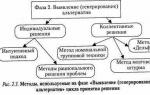
Of the existing methods for assessing the value of a company in a terminal year, appraiser consultants most often use the Gordon method, which is essentially similar to the approach based on the capitalization of income:
GV - value in the post-forecast period - at the end of the last year of the forecast period,
Cash flow of the first year of the post-forecast period,
Discount rate for the first year of the post-forecast period,
g is the long-term growth rate of cash flow in the post-forecast period.
A feature of the methods of capitalization and discounting of cash flows is that, as a rule, only one of the methods is used, which is due to the conditions of application of these approaches to valuation.
However, this does not exclude the possibility of calculating the value of a company using two methods simultaneously.
The main prerequisites for using the direct capitalization method are as follows:
The amount of current income is stable, predictable or changes at a constant growth rate, i.e. in the near future, income from the facility will remain at a level close to the current one;
A company's current performance can provide some insight into its future performance.
The method based on discounted cash flows is more appropriate when a significant change in future income compared to current income is expected, i.e. when the company's operations are expected to be materially different from current or past ones.
Particular attention should be paid to companies whose operations will decline in the future (negative growth rate) or whose economic life will cease in the near future (bankruptcy is highly likely).
In this case, the use of both methods may be questionable.
It should be noted that the approach based on discounting future cash flows is based on events that are only expected. Therefore, the value obtained using this approach directly depends on the accuracy of the forecast of the appraiser, the analyst.
This approach should not be used when there is insufficient data to form a reasonable forecast of net cash flow long enough into the future.
However, even using rough forecast metrics, an approach based on discounting future earnings streams can be useful in determining the estimated value of a company.
Among other things, the stage of the company's life cycle and industry, as well as the type of company being assessed, must be taken into account.
It is obvious that applying the capitalization method at a time of active growth of the company is unlikely to give an adequate value result.
Examples are telecommunications companies, high-tech businesses developing robotics, innovative products, companies in the process of restructuring, etc.
In addition, when capitalizing income, it is necessary to understand that not only the amount of the company’s income is transmitted to all subsequent periods, but also the structure of its capital, the rate of return, and the company’s risk level.
Thus, to choose a method for calculating value, it is necessary to understand how the company’s income or cash flows will change in the near future, analyze not only the financial condition of the company being valued and its development prospects, but also the macroeconomic situation in the world, country, or industry to which applies to the company as well as related industries.
A major role in choosing an assessment method is played by the purpose of the assessment itself and the intended use of its results.
For example, in cases where it is necessary to quickly determine the market value of a business using the income approach methods or confirm the results obtained using comparative or cost approaches, the capitalization method is optimal because it will allow you to quickly obtain a relatively reliable result.
Also, the capitalization method is justified when preparing analytical materials when a deep dive into the company’s financial flows is not required or is not possible.
An almost ideal case for using the capitalization method is a rental business.
In all other cases, especially when the income approach is the only one within which the cost is calculated, in our opinion, the discounted cash flow method is more preferable.
The Gordon model is commonly used to calculate the reversion cost (terminal value) when using the discounted cash flow (DCF) method to determine the value of non-depreciable assets. At its core, the Gordon model formula is the sum of an infinite discounted income stream. The calculated dependence has the following form:
Rev – cost of reversion;
NOR – net operating income;
Y – discount rate;
g– rate of change in the respiratory rate;
m – number of the initial period;
Abbreviation for the Gordon model formula.
For depreciating assets, such as real estate, the cost of reversion is usually determined by other methods. As one of the calculation options, the method of direct capitalization of the NPV of the first year of the post-forecast period is used. The direct capitalization (DC) method is also used as an independent method for determining the value of real estate.
However, unlike the DCF method, the PC method describes a different model of ownership of a property. This method assumes that an investor, investing in real estate, owns this object until the end of its life and at the same time accumulates funds for the subsequent acquisition, after complete depreciation, of a similar real estate object. That is, thereby deliberately reducing the amount of incoming income by the rate of return of capital. The dependence for the PC method has the following form:
Co – the cost of the property;
R – capitalization ratio;
f– rate of return of capital;
index 0 – corresponds to the date of assessment;
index 1 – corresponds to the first forecast period.
Since the PC and DCF methods reflect slightly different patterns of investor behavior, it is not surprising that, given certain initial data, they can give different results.
To demonstrate the correctness of the descriptive model of the PC method presented above, we transform dependence (2) to the following form:
Thus, we have obtained the classic formula for calculating the return on invested capital. For example, in the case of lending, the ratio of annual interest payments on the loan to the loan amount.
Since the rate of return on capital is calculated taking into account the remaining economic life of the asset (the period of capital ownership), it follows that the PC method is built on a model that assumes that the investor, after investing capital in an asset, will own it until the end of its economic life, which confirms the above.
In fairness, it should be noted that the DCF method for a non-depreciating asset that uses the Gordon model (since no return of capital is required) can also be considered as a model that assumes indefinite ownership of the asset.
Dependence (3) can be written in the following form:
If BOR = const (g = 0), the first term in dependence (4) corresponds to the formula of the Gordon model in the absence of changes in BOD. Therefore, substituting formula (1) into (4) and transforming the resulting dependence, we obtain:
Analysis of dependence (5) indicates an unexpected, at first glance, result: a depreciating asset (having a finite life) generates an infinite stream of income. This can be explained as follows. Since the PC method assumes the return of capital at the end of the asset's life in order to acquire a similar asset, then in fact the model described by the PC method assumes infinite ownership of a periodically renewed asset with a limited life.
If the BOD is const (g 0), then depending on (5) you should use
Yo – discount rate for the DCF method.
Transforming dependence (5) for this case, we obtain:
Analysis of dependence (6) allows us to conclude that the PC and DCF methods in the general case not only reflect different models of investor behavior, but are also characterized by different rates of return, which is quite logical, since different periods of ownership of an object imply different risks.
However, the fact that the rate of return for the PC method with a growing NOR is less than the discount rate for the DCF method, at first glance, does not seem entirely logical, since usually, the longer the holding period of the asset (life of the asset), the higher, in general, risk of default. This explains, for example, that in the stock market, the later the maturity date of a bond, the higher its yield. However, in the case of a depreciating asset, the opposite effect appears to be observed in that over time, as the recovery fund accumulates and the value of the asset declines, the magnitude of the loss in the event of default decreases. Consequently, the integral value of default risk in this case is lower.
In fact, the idea that when using the PC method, it is necessary to take into account the growth rate of the NRR not only in the numerator, but in the denominator was expressed, for example, in. However, the absence of an explicit formula led to the fact that in practice this point was usually not taken into account in the calculations. Apparently, in this regard, the results of calculations using the PC and DCF methods with the same initial data, in the case of non-constant NOR and the same rates of return, differed, sometimes very significantly, from each other. Moreover, the result of the PC method, with an increasing NOR, was always lower than the result of the DCF method. Taking into account the rate of growth of NRR in the denominator allows us to reduce this discrepancy in the calculation results. However, differences in results may remain due to initial differences in the models. Dependence (6) can also be recommended for use when capitalizing the NPV of the post-forecast period in the case of using the DCF method.
Chapter 2. Assessment of the market value of JSC Kalugapribor (JSC Kalugapribor)
(DCF) describes a model based on the assumption that the value of an asset is equal to the discounted sum of the income stream generated by the asset during the holding period (forecast period) and the discounted reversion value at which the asset is expected to be sold (to return the invested capital) after the end of the holding period.
The Gordon model is commonly used to calculate the reversion cost (terminal value) when using the discounted cash flow (DCF) method to determine the value of non-depreciable assets. At its core, the Gordon model formula is the sum of an infinite discounted income stream. The calculated dependence has the following form:
Rev – cost of reversion;
NOR – net operating income;
Y – discount rate;
g– rate of change in the respiratory rate;
m – number of the initial period;
Abbreviation for the Gordon model formula.
For depreciating assets, such as real estate, the cost of reversion is usually determined by other methods. As one of the calculation options, the method of direct capitalization of the NPV of the first year of the post-forecast period is used. The direct capitalization (DC) method is also used as an independent method for determining the value of real estate.
However, unlike the DCF method, the PC method describes a different model of ownership of a property. This method assumes that an investor, investing in real estate, owns this object until the end of its life and at the same time accumulates funds for the subsequent acquisition, after complete depreciation, of a similar real estate object. That is, thereby deliberately reducing the amount of incoming income by the rate of return of capital. The dependence for the PC method has the following form:
![]() (2)
(2)
Co – the cost of the property;
R – capitalization ratio;
f– rate of return of capital;
index 0 – corresponds to the date of assessment;
index 1 – corresponds to the first forecast period.
Since the PC and DCF methods reflect slightly different patterns of investor behavior, it is not surprising that, given certain initial data, they can give different results.
To demonstrate the correctness of the descriptive model of the PC method presented above, we transform dependence (2) to the following form:
![]() (3)
(3)
From here: ![]()
Thus, we have obtained the classic formula for calculating return on invested capital. For example, in the case of lending, the ratio of annual interest payments on the loan to the loan amount.
Since the rate of return on capital is calculated taking into account the remaining economic life of the asset (the period of capital ownership), it follows that the PC method is built on a model that assumes that the investor, after investing capital in an asset, will own it until the end of its economic life, which confirms the above.
In fairness, it should be noted that the DCF method for a non-depreciating asset that uses the Gordon model (since no return of capital is required) can also be considered as a model that assumes indefinite ownership of the asset.
Dependence (3) can be written in the following form:
![]() (4)
(4)
If BOR = const (g = 0), the first term in dependence (4) corresponds to the formula of the Gordon model in the absence of changes in BOD. Therefore, substituting formula (1) into (4) and transforming the resulting dependence, we obtain:
![]() (5)
(5)
Analysis of dependence (5) indicates an unexpected, at first glance, result: a depreciating asset (having a finite life) generates an infinite stream of income. This can be explained as follows. Since the PC method assumes the return of capital at the end of the asset's life in order to acquire a similar asset, then in fact the model described by the PC method assumes infinite ownership of a periodically renewed asset with a limited life.
If the BOD is const (g 0), then depending on (5) you should use
Yo – discount rate for the DCF method.
Transforming dependence (5) for this case, we obtain:
Analysis of dependence (6) allows us to conclude that the PC and DCF methods in the general case not only reflect different models of investor behavior, but are also characterized by different rates of return, which is quite logical, since different periods of ownership of an object imply different risks.
However, the fact that the rate of return for the PC method with a growing NOR is less than the discount rate for the DCF method, at first glance, does not seem entirely logical, since usually, the longer the holding period of the asset (life of the asset), the higher, in general, risk of default. This explains, for example, that in the stock market, the later the maturity date of a bond, the higher its yield. However, in the case of a depreciating asset, the opposite effect appears to be observed in that over time, as the recovery fund accumulates and the value of the asset declines, the magnitude of the loss in the event of default decreases. Consequently, the integral value of default risk in this case is lower.
In fact, the idea that when using the PC method, it is necessary to take into account the growth rate of the NRR not only in the numerator, but in the denominator was expressed, for example, in. However, the absence of an explicit formula led to the fact that in practice this point was usually not taken into account in the calculations. Apparently, in this regard, the results of calculations using the PC and DCF methods with the same initial data, in the case of non-constant NOR and the same rates of return, differed, sometimes very significantly, from each other. Moreover, the result of the PC method, with an increasing NOR, was always lower than the result of the DCF method. Taking into account the rate of growth of NRR in the denominator allows us to reduce this discrepancy in the calculation results. However, differences in results may remain due to initial differences in the models. Dependence (6) can also be recommended for use when capitalizing the NPV of the post-forecast period in the case of using the DCF method.
Conclusion
It has been proven that the Gordon model, adjusted for the rate of return of capital, can be used to determine the value of real estate and other depreciable assets using the income approach methods.
It is shown that the discount rate used in the discounted cash flow method should be used in the direct capitalization method only in an adjusted form.
Literature
1. Business valuation. Ed. , . M.: Finance and Statistics, 2002
2. Analysis and evaluation of income-generating real estate. M.: Delo, 1995, pp. 74-75.
Note.
Originally posted at http://www. *****/default. aspx? SectionId=35&Id=2974
The Gordon model, named after Myron J. Gordon, who did much to develop and popularize this method, assumes that the growth rate of the income stream in the residual period is constant.
The Gordon model's estimate of the company's residual value should be the same as the estimate that would be obtained if the residual value were estimated taking into account an unlimited forecast period. The Gordon model, of course, is preferable because it does not require cash flow forecasts for a long period of time.
Formula for estimating residual value using the Gordon model:
| Residual value | = | Дt r - g |
where: Дt- annual, stable income stream for the first year after the end of the forecast period;
r- the corresponding rate of return;
g- long-term growth rate.
Notes:
- The above formula takes into account all income streams that will be received from owning a company outside of the appraiser's forecast period.
- The residual income stream should be similar to the income stream used to value the company during the forecast period. If the appraiser has decided that the cash flow for equity capital can be reliably predicted, and therefore the company’s valuation should be based on it, then it is the cash flow for equity capital that should be used to evaluate the company’s activities, both in the forecast and in the residual period.
- The income stream and rate of return must match each other. Suppose the appraiser makes all forecasts in real terms (not taking into account inflation) and uses cash flow for equity to calculate residual value, then the rate of return on capital should be determined by a). for equity, b). excluding inflation.
- In the remaining period, when determining the amount of cash flow, capital investments must be equal to accrued depreciation. It is assumed that in the remaining period the company has reached a stable level of income and is not making large investments in expanding production. However, in order to maintain a stable level of production, it is necessary to make investments in the maintenance and replacement of existing fixed assets. Such investments include maintenance, repair, and gradual replacement of aging equipment, maintaining buildings and structures in working order, etc. If we assume that in the remaining period capital investments will be lower than depreciation, then over time the amount of depreciation will be reduced to zero, which is unlikely for the existing enterprises. If capital investment is higher than depreciation, then the income stream will never be constant.
- The rate of income growth is constant and less than the rate of return on capital. A constant revenue growth rate indicates that the company is not in a rapid growth or decline stage, but rather in a maturity stage.
The Gordon model only works if the income growth rate (g)
less than the rate of return on capital (r).
As a rule, investors (owners) expect that the income from owning companies will increase every year. While revenue growth rates vary among companies, it is very common for investors to make long-term growth forecasts based on projected gross domestic product (GDP) growth rates. Appraisers, if they can find reliable data, use forecasts of long-term growth rates, both for the industry as a whole and specifically for the company being valued. The long-term growth rate of the company under evaluation can be determined based on the analysis of data from past years, and it is necessary to take into account at what stage of the life cycle the company as a whole or the individual goods and services it produced was at. The most preferred method of estimating growth rate is the overall industry growth expectation, since no company can sustain a higher growth rate than the industry average over a long period.
The expected growth rate (g) should take into account:
1. Inflationary price increases (if forecasts are made taking into account inflation)
2. Growth in production and sales:
· industry average growth;
· growth at the enterprise being assessed exceeds the industry average growth.
Some estimators, when making forecasts taking into account inflation, assume that in the remaining period the rate of income growth will be equal to inflation, then g is the percentage of inflation.
If the estimator predicts no growth in the remainder of the period, even due to inflation (this situation is possible if forecasts are made in real terms), then the formula for the Gordon model is as follows:
This task shows how sensitive the residual value is to a given growth rate. So, when the growth rate changed by 4%, the residual value increased by 24%, and when the growth rate changed by 8%, the residual value increased by 59%.
The diagram below shows this relationship.
Liquidation value
The liquidation value method assumes that the residual value is equal to the proceeds from the sale of assets owned by the company less the payment of any liabilities that will arise at the end of the forecast period. The residual value obtained by this method is usually far from the value obtained based on the Gordon model. If the industry to which the company being valued belongs is growing and profitable, then the residual value calculated on the basis of liquidation value will be significantly lower than the residual value calculated on the basis of the Gordon model. In an industry experiencing a decline, the liquidation value, on the contrary, may be higher. The residual value of the company needs to be calculated only in the only case when at the end of the forecast period the company, however, will be liquidated. This situation is possible if a company was created, for example, to develop a mine, and after the reserves of raw materials are exhausted, the company will cease to exist. In this case, the company's forecast period will last as long as the production of raw materials at the mine generates positive cash flow, after which the company will be liquidated. Calculating the residual value of a company based on its liquidation value is associated with the difficulty of forecasting 1). the liquidation value of assets, the liquidation of which is significantly removed in time from the valuation date, and 2). amounts of liabilities.
Net asset value
This method differs from the previous one only in that at the end of the forecast period, income from the sale of assets, as well as liabilities, are determined by their market value at that time.
Replacement cost
This method states that the residual value of a company is equal to the projected cost of replacing the company's assets. This method has a large number of disadvantages. The most significant ones are listed below:
Only tangible assets are subject to replacement. So-called "organizational capital" can only be assessed on the basis of the income it generates. Estimating the residual value at the replacement cost of tangible assets can lead to a significant undervaluation of the company.
Not all company assets are replaceable. Let's imagine equipment that can only be used in a specific industry. The cost of replacing an asset may be so high that it makes replacement uneconomic. And, as long as the asset generates positive cash flow, it has value to the going concern.
Price/earnings multiple
The method assumes that in the residual period the value of the company will be equal to some multiplier of its future profits that will arrive in the residual period. This statement is true. The difficulty lies in determining the size of this multiplier. Let's assume that we know the industry average price/earnings multiple at the current time. The value of the multiplier reflects investors' expectations regarding the development prospects of the company and the industry, both in the forecast and in the remaining period. However, the same prospects at the end of the forecast period may differ significantly from today. Therefore, to estimate the residual value, a different Price/Earnings multiple is needed, which would reflect the company's prospects at the end of the forecast period. What indicators will determine the value of this multiplier? These are the same factors that influence the residual value calculated using the Gordon model: expected growth rate, return on newly invested capital and rate of return on capital. Thus, it is better to use the Gordon model to estimate the residual value of a business, since this model takes into account current expectations of key indicators, and not their possible values at the end of the forecast period.
Price/Book Value Multiplier
The method assumes that in the remaining period the value of the company will be equal to some multiplier of the book value of its assets. Often, for the residual period, the current value of the multiplier for the company being valued or the average multiplier of peer companies is used. The application of this method to assess the residual value of a company is associated with the same problems as in the case of the application of the previous method. In addition to the problems associated with determining the multiple at some distant point in the future, the book value of assets is itself distorted by the effects of inflation and is affected by accounting rules.
DISCOUNTING FACTOR
Since all projected cash flows will be available to the owners at some point in the future, to determine the value of the company at the valuation date, it is necessary to discount them (reduce them to the valuation date). The discounting process is discussed in detail in the manual by K.Yu. Stabrovskaya. "Six functions of compound interest."
To determine the current value of cash flow received in period (planning interval) n (CFn), it is necessary to multiply the cash flow of a given period by the discount factor calculated for this period.
In textbooks on the theory of real estate valuation, you can find the following formula for calculating the discount factor:
| Fn | = | (1+r)n |
Where: r is the rate of return on capital;
n - annual planning interval.
The discount factor calculated using this formula is called the end-of-period discount factor. By discounting cash flows using the discount factor for the end of the period, the appraiser assumes that absolutely all of the enterprise’s flows (receipt of gross income, payment of operating expenses, etc.) occur at one point in time - at the end of each planning interval. For an enterprise, such an assumption is even less likely than for real estate. In this regard, in the theory of business valuation, to determine the current value of cash flows, a discount factor for the middle of the period is used, which is calculated by the formula:
| Fn | = | (1 + r) n-0.5 |
In this case, it is assumed that cash inflows and outflows seem to occur in the middle of the planning interval. In fact, of course, cash inflows and outflows at an enterprise occur more or less evenly throughout the entire planning interval. By applying a discount factor to the middle of the period, the appraiser more accurately reflects the situation of uniformity of cash inflows and outflows at enterprises.
Related information.
Dividend discounting is one of the simplest ways to roughly estimate the value of a stock. This valuation model (discount dividend model, DDM) is based on the concept. In accordance with it, the value of a share is equal to the value of future dividends reduced (discounted) to the current point in time. Simply put, you forecast the company's future dividends and discount them to arrive at the fair value of the stock. If the market price of a stock is below its fair value, the stock is undervalued.
To value a stock using the dividend discount model, you will need:
- current dividends
- their expected growth rates
- discount rate
In general, the DDM formula looks like this: ![]()
div — expected dividends per share
k — discount rate
P — fair share price
If dividend growth is expected, the formula is converted to the following form:
DPS0 - current dividend
g—expected growth rate
If the life of the company is assumed to be infinite, then the formula transforms into the so-called Gordon formula - a model of constant growth.

P forecasting future dividends
To forecast future cash flows, you need to multiply the current dividend by the expected growth rate g. Current dividends can be found in mine, on the company’s official website or on other sites that I mentioned. Next year's dividend is calculated using the formula
D1=D0*(1+g)
For example, in the last year D0 was 1 ruble, the expected growth rate is 15%, then next year D1 will be equal to 1*(1+0.15)=1.15.
Rates of growth
Most companies have dividends that grow over time. To find out their future value, it is necessary to assume at what rate they will grow. To estimate future growth rates you can:
- take the average growth rates in the past if they were stable (my table will help here again)
- calculate using formula
g = ROE*b
ROE (return on equity)— return on equity = net profit/equity
b— the reinvested profit ratio, that is, the share of profit that the company retains for itself after paying dividends. b = 1 — (amount of dividends paid/net profit). Sometimes the share of profits that is paid out to shareholders is specified in the company's dividend policy. For example, it is known that Nizhnekamskneftekhim and Kazanorgsintez pay shareholders 30% of the private equity, which means the share of reinvested profit is 70%.
Discount rate
The discount rate can be calculated in different ways. Essentially this is the rate of return required. That is, if you want to receive a 15% return on your investment, then take this rate. Another way is to use the CAPM (Capital Asset Pricing Model). According to it, the discount rate is calculated as
R = R(f) + β * Risk Premium
R—required rate of return
R(f) is the risk-free rate of return. Yield can be used. You can view current market rates on the website of the Central Bank of the Russian Federation.
β (beta) is a coefficient characterizing the measure of market risk of shares. The more a stock's performance deviates from the index's performance to a greater or lesser extent, the riskier it is considered. Calculating this coefficient manually is very labor-intensive, but it can be found on the Infestfunds website. I personally do not use this coefficient in my calculations for my personal reasons.
Risk Premium - risk premium - premium for the risk of investing in shares, equal to the historical difference between the return of the stock market and the return of risk-free instruments. If , then over the past 10 years the risk premium for equities has been 3.2% compared to government bonds. If we compare over 15 years with deposits, then it is already 7.5%. Another option to view the premium risk by country is in the Damodaran table.
The current OFZ yield is about 10%, let's take the risk premium at 5%. Then R = 10+5=15%. You are free to take any rate of return that your mind and intuition tells you; it is not necessary to use CAPM. But the higher the bet, the lower the stock's valuation will be.
Application of the dividend discount model
The application of the model depends on three scenarios:
- zero dividend growth rate
- constant growth rate
- growth rate changes over time
Let us now consider each scenario separately.
Growth rate is zero
An example of the first option, when dividends do not grow, is the preferred shares of Kazanorgsintez. They pay out 25 kopecks per share annually if there is net profit.

In this case, the fair price of the share, if we apply a discount rate of 15%, is equal to P = 0.25/0.15 = 1.66 rubles.
Constant growth rate
Some stocks have very stable growth rates in the past and are expected to continue to do so in the future. For example, MTS has reached its ceiling and one cannot expect strong growth in the long term. This model uses the Gordon formula, which assumes dividends will flow forever. No company can maintain high growth rates forever; they eventually tend to the economic average. Let's assume that MTS's long-term growth rate is 5% per year.

First, we calculate the next year's dividend, for this we use the formula D1=D0*(1+g).
25.76*(1+0.05)=27.04 rubles
To calculate the fair price of a stock, we use the Gordon formula
P = 27.04/(0.15-0.05) = 270.48 rubles.
This model has a number of disadvantages. If we take too high a growth rate, which is greater than the discount rate, the result will be negative. Therefore, it is only suitable for cases where g is less than k and is used to evaluate mature companies.
Inconsistent dividend growth
Most stocks have variable dividend growth rates over time. No company can increase its payout to shareholders by 30-40% per year forever. Usually, over time, high growth rates fall to some lower and more stable ones. For example, the dividends of such an old and large company as Coca-Cola are now growing by an average of 9% per year.
For example, let's take dividends, which will grow by 17% per year for the first 10 years, then by 5% per year forever. To do this, they must be discounted for each period and then summed up. Let's take a discount rate of 15%. The current dividend is 20 rubles.
First, let's discount the cash flows for the first 10 years. Let's build a table for this.
| Year | Calculation | Dividend |
| 0 | 20 | 20,00 |
| 1 | 20*(1+0,17)^1 | 23,40 |
| 2 | 20*(1+0,17)^2 | 27,38 |
| 3 | 20*(1+0,17)^3 | 32,03 |
| 4 | 20*(1+0,17)^4 | 37,48 |
| 5 | 20*(1+0,17)^5 | 43,85 |
| 6 | 20*(1+0,17)^6 | 51,30 |
| 7 | 20*(1+0,17)^7 | 60,02 |
| 8 | 20*(1+0,17)^8 | 70,23 |
| 9 | 20*(1+0,17)^9 | 82,17 |
| 10 | 20*(1+0,17)^10 | 96,14 |
Now we discount them at a rate of 15%.
| 23,4/(1+0,15)^1 | 20,34 |
| 27,38/(1+0,15)^2 | 20,70 |
| 32,03/(1+0,15)^3 | 21,06 |
| 37,48/(1+0,15)^4 | 21,42 |
| 43,85/(1+0,15)^5 | 21,80 |
| 51,3/(1+0,15)^6 | 22,17 |
| 60,02/(1+0,15)^7 | 22,56 |
| 70,23/(1+0,15)^8 | 22,95 |
| 82,17/(1+0,15)^9 | 23,35 |
| 96,14/(1+0,15)^10 | 23,76 |
| Sum | 220,16 |
Now let's calculate the value of the stock after the first 10 years (terminal value). Let's take the cash flow for year 10 and use Gordon's formula. The terminal value of the share after the first 10 years will be 96.14*1.05/(0.15-0.05)=1009.47. Let's discount it to the current moment 1009.47/(1+0.15)^10=249.52.
The total cost of the share will be 220.16+249.52=469.68.
Discounting Dividends in Excel
To avoid making all these calculations manually, you can use Excel. To do this, plot future cash flows in a column, select the NPV (net present value) function, enter the discount rate and values. The result will be the same.

Dividend discounting using an example.
Let's take Acron stock as an example. The current dividend is 139 rubles. Average dividend growth rate over 10 years is 17%.

The company is not characterized by stable profitability, but the average ROE over 8 years is about 20%. Acron pays 30% of net profit in dividends (more in 2013 and 2014), so the share of reinvested profit is 70%. We calculate the expected growth rate of 0.2*0.7=0.14 or 14%. Let's take a discount rate of 15%.
If dividends do not increase further, then the share price is 139/0.15 = 926 rubles.
If dividends grow forever by 5% per year, then the share price is 139 * 1.05 / (0.15-0.05) = 1459.5 rubles.
Now let's depict a three-stage growth model: for the first 5 years, dividends will grow by 14%, the second five years by 10%, and the rest of the time by 5%.
To do this, we will build a cash flow table in Excel.
 NPV is the net present value of dividends for the first 10 years. PV is the terminal value of the stock in 10 years, calculated using the Gordon formula. DTS is the discounted terminal value of the stock at the current moment. Value is the fair value of the share.
The market price of the share is 2590. That is, either the share is overvalued, or we made a mistake in the calculations, for example, we assumed too low growth rates. Given the devaluation of the ruble, the market is now factoring into the share price a significant increase in profits for 2015, and therefore dividends next year. The average dividend yield of Acron shares over 5 years was 8.4%. If the market expects a similar dividend in 2016, then it turns out that it expects dividends in the amount of 217 rubles.
Disadvantages of the model
- Suitable only for dividend paying stocks.
- Does not take into account a possible increase in the market value of shares.
- Highly dependent on the discount rate applied and projected cash flows. A slight change in input data leads to a significant change in the result.
- Well suited for companies with stable financial performance (profitability, net profit growth), and poorly suited for companies with unstable results.
- It does not take into account factors such as: future share buybacks and additional issues, changes in the share of paid profits, rise and fall in prices for raw materials and products, changes in the debt burden and investment program, and so on. Some of this can only be taken into account manually by forecasting profits and dividends for each period.